Equilibrium by Entropy Maximisation

Thermodynamics and Statistical Mechanics

P. Attard

Preface

Thermodynamics deals with the general principles and laws that govern the behaviour of matter and with the relationships between material properties. The origins of these laws and quantitative values for the properties are provided by statistical mechanics, which analyses the interaction of molecules and provides a detailed description of their behaviour. This book presents a unified account of equilibrium thermodynamics and statistical mechanics using entropy and its maximisation.

A physical explanation of entropy based upon the laws of probability is introduced. The equivalence of entropy and probability that results represents a return to the original viewpoint of Boltzmann, and it serves to demonstrate the fundamental unity of thermodynamics and statistical mechanics, a point that has become obscured over the years. The fact that entropy and probability are objective consequences of the mechanics of molecular motion provides a physical basis and a coherent conceptual framework for the two disciplines. The free energy and the other thermodynamic potentials of thermodynamics are shown simply to be the total entropy of a subsystem and reservoir; their minimisation at equilibrium is nothing but the maximum of the entropy mandated by the second law of thermodynamics and is manifest in the peaked probability distributions of statistical mechanics. A straightforward extension to nonequilibrium states by the introduction of appropriate constraints allows the description of fluctuations and the approach to equilibrium, and clarifies the physical basis of the equilibrium state. Although this book takes a different route to other texts, it shares with them the common destination of explaining material properties in terms of molecular motion. The final formulae and interrelationships are the same, although new interpretations and derivations are offered in places. The reasons for taking a detour on some of the less-travelled paths of thermodynamics and statistical mechanics are to view the vista from a different perspective, and to seek a fresh interpretation and a renewed appreciation of well-tried and familiar results. In some cases this reveals a shorter path to known solutions, and in others the journey leads to the frontiers of the disciplines. The book is basic in the sense that it begins at the beginning and is entirely self-contained. It is also comprehensive and contains an account of all of the modern techniques that have proven useful in modern equilibrium, classical statistical mechanics. The aim has been to make the subject matter broadly accessible to advanced students, whilst at the same time providing a reference text for graduate scholars and research scientists active in the field. The later chapters deal with more advanced applications, and while their details may be followed step-by-step, it may require a certain experience and sophistication to appreciate their point and utility. The emphasis throughout is on fundamental principles and upon the relationship between various approaches. Despite this, a deal of space is devoted to applications, approximations, and computational algorithms; thermodynamics and statistical mechanics were in the final analysis developed to describe the real world, and while their generality and universality are intellectually satisfying, it is their practical application that is their ultimate justification. For this reason a certain pragmatism that seeks to convince by physical explanation rather than to convict by mathematical sophistry pervades the text; after all, one person's rigor is another's mortis. The first four chapters of the book comprise statistical thermodynamics. This takes the existence of weighted states as axiomatic, and from certain physically motivated definitions, it deduces the familiar thermodynamic relationships, free energies, and probability distributions. It is in this section that the formalism that relates each of these to entropy is introduced. The remainder of the book comprises statistical mechanics, which in the first place identifies the states as molecular configurations, and shows the common case in which these have equal weight, and then goes on to derive the material thermodynamic properties in terms of the molecular ones. In successive chapters the partition function, particle distribution functions, and system averages, as well as a number of applications, approximation schemes, computational approaches, and simulation methodologies, are discussed. Appended is a discussion of the nature of probability. The paths of thermodynamics and statistical mechanics are well-travelled and there is an extensive primary and secondary literature on various aspects of the subject. Whilst very many of the results presented in this book may be found elsewhere, the presentation and interpretation offered here represent a sufficiently distinctive exposition to warrant publication. The debt to the existing literature is only partially reflected in the list of references; these in general were selected to suggest alternative presentations, or further, more detailed, reading material, or as the original source of more specialised results. The bibliography is not intended to be a historical survey of the field, and, as mentioned above, an effort has been made to make the book self-contained. At a more personal level, I acknowledge a deep debt to my teachers, collaborators, and students over the years. Their influence and stimulation are impossible to quantify or detail in full. Three people, however, may be fondly acknowledged: Pat Kelly, Elmo Lavis, and John Mitchell, who in childhood, school, and PhD taught me well.

http://personal.chem.usyd.edu.au/Phil.Attard/TDSM/preface.html

Héctor A. Chacón C.

statistical mechanics: quantitative study of systems consisting of a large number of interacting elements, such as the atoms or molecules of a solid, liquid, or gas, or the individual quanta of light (see photon photon (fō`tŏn), the particle composing light and other forms of electromagnetic radiation , sometimes called light quantum.
..... Click the link for more information. ) making up electromagnetic radiation. Although the nature of each individual element of a system and the interactions between any pair of elements may both be well understood, the large number of elements and possible interactions can present an almost overwhelming challenge to the investigator who seeks to understand the behavior of the system. Statistical mechanics provides a mathematical framework upon which such an understanding may be built. Since many systems in nature contain large number of elements, the applicability of statistical mechanics is broad. In contrast to thermodynamics Carnot cycle after the French physicist Sadi Carnot , who first discussed the implications of such cycles. During the Carnot cycle occurring in the operation of a heat engine, a definite quantity of heat is absorbed from a reservoir at high temperature; part of this heat is
..... Click the link for more information. , which approaches such systems from a macroscopic, or large-scale, point of view, statistical mechanics usually approaches systems from a microscopic, or atomic-scale, point of view. The foundations of statistical mechanics can be traced to the 19th-century work of Ludwig Boltzmann, and the theory was further developed in the early 20th cent. by J. W. Gibbs. In its modern form, statistical mechanics recognizes three broad types of systems: those that obey Maxwell-Boltzmann statistics, those that obey Bose-Einstein statistics Bose-Einstein statistics, class of statistics that applies to elementary particles called bosons, which include the photon , pion , and the W and Z particles .
..... Click the link for more information. , and those that obey Fermi-Dirac statistics Fermi-Dirac statistics, class of statistics that applies to particles called fermions. Fermions have half-integral values of the quantum mechanical property called spin and are "antisocial" in the sense that two fermions cannot exist in the same state.
..... Click the link for more information. . Maxwell-Boltzmann statistics apply to systems of classical particles, such as the atmosphere, in which considerations from the quantum theory quantum theory, modern physical theory concerned with the emission and absorption of energy by matter and with the motion of material particles; the quantum theory and the theory of relativity together form the theoretical basis of modern physics.
..... Click the link for more information.  are small enough that they may be ignored. The other two types of statistics concern quantum systems: systems in which quantum-mechanical properties cannot be ignored. Bose-Einstein statistics apply to systems of bosons (particles that have integral values of the quantum mechanical property called spin); an unlimited number of bosons can be placed in the same state. Photons, for instance, are bosons, and so the study of electromagnetic radiation, such as the radiation of a black body black body, in physics, an ideal black substance that absorbs all and reflects none of the radiant energy falling on it. Lampblack, or powdered carbon, which reflects less than 2% of the radiation falling on it, approximates an ideal black body.
..... Click the link for more information.  involves the use of Bose-Einstein statistics. Fermi-Dirac statistics apply to systems of fermions (particles that have half-integral values of spin); no two fermions can exist in the same state. Electrons are fermions, and so Fermi-Dirac statistics must be employed for a full understanding of the conduction of electrons in metals. Statistical mechanics has also yielded deep insights in the understanding of magnetism magnetism, force of attraction or repulsion between various substances, especially those made of iron and certain other metals; ultimately it is due to the motion of electric charges.
..... Click the link for more information. , phase transitions, and superconductivity superconductivity, abnormally high electrical conductivity of certain substances. The phenomenon was discovered in 1911 by Kamerlingh Onnes, who found that the resistance of mercury dropped suddenly to zero at a temperature of about 4.2&degK;.
..... Click the link for more information. .

The Columbia Electronic Encyclopedia® Copyright © 2007, Columbia University Press. Licensed from Columbia University Press. All rights reserved. www.cc.columbia.edu/cu/cup/

---

statistical mechanics

Branch of physics that combines the principles and procedures of statistics with the laws of both classical mechanics and quantum mechanics. It considers the average behaviour of a large number of particles rather than the behaviour of any individual particle, drawing heavily on the laws of probability, and aims to predict and explain the measurable properties of macroscopic (bulk) systems on the basis of the properties and behaviour of their microscopic constituents.

For more information on statistical mechanics, visit Britannica.com. Britannica Concise Encyclopedia. Copyright © 1994-2008 Encyclopædia Britannica, Inc.

---

statistical mechanics [stə′tis·tə·kəl mi′kan·iks]

(physics)

That branch of physics which endeavors to explain and predict the macroscopic properties and behavior of a system on the basis of the known characteristics and interactions of the microscopic constituents of the system, usually when the number of such constituents is very large. Also known as statistical thermodynamics.

McGraw-Hill Dictionary of Scientific & Technical Terms, 6E, Copyright © 2003 by The McGraw-Hill Companies, Inc.

---

Statistical mechanics

That branch of physics which endeavors to explain the macroscopic properties of a system on the basis of the properties of the microscopic constituents of the system. Usually the number of constituents is very large. All the characteristics of the constituents and their interactions are presumed known; it is the task of statistical mechanics (often called statistical physics) to deduce from this information the behavior of the system as a whole.

Scope

Elements of statistical mechanical methods are present in many widely separated areas in physics. For instance, the classical Boltzmann problem is an attempt to explain the thermodynamic behavior of gases on the basis of classical mechanics applied to the system of molecules.
Statistical mechanics gives more than an explanation of already known phenomena. By using statistical methods, it often becomes possible to obtain expressions for empirically observed parameters, such as viscosity coefficients, heat conduction coefficients, and virial coefficients, in terms of the forces between molecules. Statistical considerations also play a significant role in the description of the electric and magnetic properties of materials. See Boltzmann statistics, Intermolecular forces, Kinetic theory of matter
If the problem of molecular structure is attacked by statistical methods, the contributions of internal rotation and vibration to thermodynamic properties, such as heat capacity and entropy, can be calculated for models of various proposed structures. Comparison with the known properties often permits the selection of the correct molecular structure.
Perhaps the most dramatic examples of phenomena requiring statistical treatment are the cooperative phenomena or phase transitions. In these processes, such as the condensation of a gas, the transition from a paramagnetic to a ferromagnetic state, or the change from one crystallographic form to another, a sudden and marked change of the whole system takes place. See Phase transitions
Statistical considerations of quite a different kind occur in the discussion of problems such as the diffusion of neutrons through matter. In this case, the probability of the various events which affect the neutron are known, such as the capture probability and scattering cross section. The problem here is to describe the physical situation after a large number of these individual events. The procedures used in the solution of these problems are very similar to, and in some instances taken over from, kinetic considerations. Similar problems occur in the theory of cosmic-ray showers.
It happens in both low-energy and high-energy nuclear physics that a considerable amount of energy is suddenly liberated. An incident particle may be captured by a nucleus, or a high-energy proton may collide with another proton. In either case, there is a large number of ways (a large number of degrees of freedom) in which this energy may be utilized. To survey the resulting processes, one can again invoke statistical considerations. See Scattering experiments (nuclei)
Of considerable importance in statistical physics are the random processes, also called stochastic processes or sometimes fluctuation phenomena. The brownian motion, the motion of a particle moving in an irregular manner under the influence of molecular bombardment, affords a typical example. The stochastic processes are in a sense intermediate between purely statistical processes, where the existence of fluctuations may safely be neglected, and the purely atomistic phenomena, where each particle requires its individual description. See Brownian movement
All statistical considerations involve, directly or indirectly, ideas from the theory of probability of widely different levels of sophistication. The use of probability notions is, in fact, the distinguishing feature of all statistical considerations.

Methods

For a system of N particles, each of the mass m, contained in a volume V, the positions of the particles may be labeled x₁, y₁, z₁, …, x_N, y_N, z_N, their cartesian velocities v_x1, …, v_zN, and their momenta P_x1, …, P_zN. This simplest statistical description concentrates on a discussion of the distribution function f(x,y,z;v_x,v_y,v_z;t). The quantity f(x,y,z;v_x,v_y,v_z;t) ċ (dxdydzdv_xdv_ydv_z) gives the (probable) number of particles of the system in those positional and velocity ranges where x lies between x and x + dx; v_x between v_x and v_x + dv_x, and so on. These ranges are finite.
Observations made on a system always require a finite time; during this time the microscopic details of the system will generally change considerably as the phase point moves. The result of a measurement of a quantity Q will therefore yield the time average, as in Eq. (1). The integral is along the trajectory

(1) 

in phase space; Q depends on the variables x₁, …, P_zN, and t. To evaluate the integral, the trajectory must be known, which requires the solution of the complete mechanical problem.
Ensembles. J. Willard Gibbs first suggested that instead of calculating a time average for a single dynamical system, a collection of systems, all similar to the original one, should instead be considered. Such an ensemble of systems is to be constructed in harmony with the available knowledge of the single system, and may be represented by an assembly of points in the phase space, each point representing a single system. If, for example, the energy of a system is precisely known, but nothing else, the appropriate representative example would be a uniform distribution of ensemble points over the energy surface, and no ensemble points elsewhere. An ensemble is characterized by a density function ρ(x₁, …,z_N; p_x1, …,p_zN;t) ≡ p(x,p,t). The significance of this function is that the number of ensemble systems dN_e contained in the volume element dx₁ … dz_N; dp_x … dp_zN of the phase space (this volume element will be called dΓ) at time t is as given in Eq. (2).

(2) 

The ensemble average of any quantity Q is given

(3) 

by Eq. (3). The basic idea now is to replace the time average of an individual system by the ensemble average, at a fixed time, of the representative ensemble. Stated formally, the quantity defined by Eq. (1), in which no statistics is involved, is identified with defined by Eq. (3), in which probability assumptions are explicitly made.
Relation to thermodynamics. It is certainly reasonable to assume that the appropriate ensemble for a thermodynamic equilibrium state must be described by a density function which is independent of the time, since all the macroscopic averages which are to be computed as ensemble averages are time-independent.
The so-called microcanonical ensemble is defined by Eq. (4a), where c is a constant, for the energy E between E₀ and E₀ + ΔE; for other energies Eq. (4b)

(4{\it a}) 

(4{\it b}) 

holds. By using Eq. (3), any microcanonical average may be calculated. The calculations, which involve integrations over volumes bounded by two energy surfaces, are not trivial. Still, many of the results of classical Boltzmann statistics may be obtained in this way. For applications and for the interpretation of thermodynamics, the canonical ensembles is much more preferable. This ensemble describes a system which is not isolated but which is in thermal contact with a heat reservoir.
There is yet another ensemble which is extremely useful and which is particularly suitable for quantum-mechanical applications. Much work in statistical mechanics is based on the use of this so-called grand canonical ensemble. The grand ensemble describes a collection of systems; the number of particles in each system is no longer the same, but varies from system to system. The density function p(N,p,x) dΓ_N gives the probability that there will be in the ensemble a system having N particles, and that this system, in its 6N-dimensional phase space Γ_N, will be in the region of phase space dΓ_N.

McGraw-Hill Concise Encyclopedia of Physics. © 2002 by The McGraw-Hill Companies, Inc.

http://encyclopedia2.thefreedictionary.com/statistical+mechanics

Héctor A. Chacón C.

Thermodynamics - Terminology

Thermodynamics is the branch of science that deals with the conversions of various forms of energy and the effect on the state of a system. It was developed in the 19^th century, when it was of great practical importance in the era of steam engines. Since the microscopic structure of matter is not known at that time, it can only prescribe a macroscopic view. It remains valid and useful in the 21^th century, but now we understand such macroscopic description is just the averaged behaviour of a large collection of microscopic constituents. 

It is essential to define the terminology before learning more about the subject:
• Heat - Heat (Q) is a form of energy transfer associated with random motion of the microscopic particles.
• Work - Work (W) is the organized form of energy transfer associated with the motion of microscopic particles as a whole (in a certain direction), e.g., the expanding gas that propels a piston.
• Internal Energy - The internal energy (U) of a system is the total energy due to the motion of molecules, plus the rotation, and vibration of atoms within molecules. Heat and work are two methods of adding energy to or subtracting energy from a system. They represent energy in transit and are the terms used when energy is moving. Once the transfer of energy is over, the system is said to have undergone a change in internal energy dU. Thus, in terms of the amount of heat dQ and work dW:
  
  dU = dQ + dW ---------- (1)
  
  where dQ and dW are positive for energy transfer from the surroundings to the system, and negative for energy transfer from the system to the surroundings. If the process of energy transfer is broken down into finer details, e.g., change in disorder (dS), volume expansion/contraction (dV), and adding a new species of particles (dN), then the change in internal energy can be expressed as:
  
  dU = T dS - p dV + dN ---------- (2)
  
  where is the chemical potential.
  
  
• Free Energy - The amount of available energy that is capable of performing work.
• Temperature - Temperature (T) is related to the amount of internal energy in a system. As more heat or work is added the temperature rises, similarly a decrease in temperature corresponds to a loss of heat or work performed from the system. Temperature is an intrinsic property of a system, meaning that it does not depend on the system size or the amount of material in the system. Other intrinsic properties include pressure and density. The internal energy (U) is related to the temperature (T) by the formula:
  
  U= (3nR/2) T ---------- (3)
  
  where R = 8.314x107 erg/K^o-mole is called the gas constant.
• Pressure - Pressure (p) is the force normal to the surface of area upon which it exerts. Microscopically, it is the transfer of momenta from the particles that produces the force on the surface.
• Volume - Volume (V) is referred to the three dimensional space occupied by the system.
• Particle Number - Particle number (N) is the number of a particular constituents in a system.
• Avogadro's Number - Avogadro's number (N₀) is 6.023 x 10²³. One mole is defined as the unit that contains that many number of particles such as atoms, molecules, or ions, e.g., it is the number of carbon-12 atoms in 12 gram of the substance, or the number of protons in 1 gram of the same substance, etc.
• Number of Moles - Number of moles (n) is the number of particles in the unit of a mole, i.e., n = N / N₀.
• Density - Density () is defined as mass per unit volume.
• Entropy - Entropy (S) is a measure of disorder in the system. Mathematically, the change of entropy dS is related to the amount of heat transfer dQ by the formula:
  
  dS = dQ / T    or    dQ = T dS ---------- (4)
  
  
• Chemical Potential - The chemical potential () of a thermodynamic system is the change in the energy of the system when a different kind of constituent particle is introduced, with the entropy and volume held fixed.

Some thermodynamics definitions here such as temperature, pressure, and density are specified under an equilibrium condition. The changes in these variables are idealized with a succession of equilibrium states. Many important biochemical and physical

processes (such as in microfluid, chemical reactions, molecular folding, cell membranes, and cosmic expansion) operate far from equilibrium, where the standard theory of thermodynamics does not apply. Figure 01a shows the cases for different kinds of thermodynamic theory. Case 1 is for over all equilibrium in the system, which is described by classical thermodynamics. Case 2 has local equilibrium in different regions. A theory of nonequilibrium thermodynamics (using the concept of flow or flux) has been developed for such situation. In case 3 the molecules become a chaotic jumble such that the concept of

Figure 01a Thermodynamics Theory [view large image]

temperature is not applicable anymore. A new theory has been formulated by using a new set of variables within the very short timescale for the transformation. The second law of thermodynamics has been shown to be valid for all these cases.

[Top]

---

The Four Laws of Thermodynamics

• Zeroth law - It is the definition of thermodynamic equilibrium. When two systems are put in contact with each other, energy and/or matter will be exchanged between them unless they are in thermodynamic equilibrium. In other word, two systems are in thermodynamic equilibrium with each other if they stay the same after being put in contact.
  
  The original zeroth law is stated as If A and B are in thermodynamic equilibrium, and B and C are in thermodynamic equilibrium, then A and C are also in thermodynamic equilibrium.
  
  Thermodynamic equilibrium includes thermal equilibrium (associated to heat exchange and parameterized by temperature), mechanical equilibrium (associated to work exchange and parameterized generalized forces such as pressure), and chemical equilibrium (associated to matter exchange and parameterized by chemical potential).
• 1st Law - This is the law of energy conservation. It is stated alternatively in many forms as follows:
  
  The work exchanged in an adiabatic process depends only on the initial and the final state and not on the details of the process.
  or
  The heat flowing into a system equals the increase in internal energy of the system minus the work done by the system.
  or
  Energy cannot be created, or destroyed, only modified in form.
  
  The second statement can be expressed mathematically in the form of Eq.(1) with negative W representing work done by the system. The adiabatic process in the first statement refers to a system with no heat transfer, i.e., Q = 0.

2nd Law - It can be stated in many ways, the most popular of which is: It is impossible to obtain a process such that the unique effect is the subtraction of a positive heat from a reservoir and the production of a positive work. or A system operating in a cycle cannot produce a positive heat flow from a colder body to a hotter body. The first statement is to exclude the un-realistic situations such as to drive a steamship across the ocean by extracting heat from the water, or to run a power plant by extracting heat from the surrounding air. The second statement expresses the impossibility of running refrigeration without work. Another form of the 2nd law states:

Figure 01b Entropy, Addition [view large image]

The entropy of an isolated system tends to remain constant or to increase. It is in this form that the arrow of time is defined. Figure 01b shows the various ways entropy can be added to a system.

• 3rd Law: This law explains why it is so hard to cool something to absolute zero:
  
  All processes cease as temperature approaches zero.
  
  This statement is expressed mathematically by Eq.(4), which shows that as the temperature T approaches zero the amount of heat extracted from the system also diminishes to zero. Thus, even using laser cooling would not be able to attain a temperature of absolute zero.

[Top]

---

Systems

A thermodynamic system is that part of the universe that is under consideration. A real or imaginary boundary separates the system from the rest of the universe, which is referred to as the environment. A useful classification of thermodynamic systems is based on the nature of the boundary and the flows of matter, energy and entropy through it.

There are three kinds of system depending on the kinds of exchanges taking place between a system and its environment:
1. Isolated System - It does not exchange heat, matter or work with the environment. An example of an isolated system would be an insulated container, such as an insulated gas cylinder. In reality, a system can never be absolutely isolated from its environment, because there is always at least some slight coupling, even if only via minimal gravitational attraction. Figure 02 shows the essence of classical thermodynamics: In a system isolated from the outside world, heat
   
   

   	within a gas of temperature, T2, will flow in time, t, toward a gas of temperature, T1, where T2 > T1 and T = T2 - T1, thus the system's total energy E is constant (via the first law of thermodynamics), while its free energy F decreases, and its entropy S rises (via the second law of thermodynamics), until finally T 0 at equilibrium.
   Figure 02 Isolated System [view large image]	Some literatures refer the isolated system as closed system, while the other systems are lumped together as open system.

2. Closed System - It exchanges energy (heat and work) but not matter with the environment. A greenhouse is an example of a closed system exchanging heat but not work with its environment. Another example is the heat engine shown in Figure 03. It is defined as a device that converts heat energy into mechanical energy or more exactly a system which
   
   

   	operates with only heat and work passing across its boundaries. As work is done on the gas inside the chamber, the temperature and pressure increase and some heat will be transferred out of the system. When heat is transferred to the system, the gas expands, it does work on the surroundings and the temperature and pressure decrease.
   Figure 03 Closed System [view large image]

3. Open System - It exchanges energy (heat and work) and matter with the environment. A boundary allowing matter exchange is called permeable. It's possible for an open system to import order and export disorder, locally increasing order. What the Second Law says is that in such a transaction more disorder than order will be created. It does not, however, forbid the creation of pockets of order. What happens is that disorder in the entire system will increase even though individual open systems within it might become more ordered. As shown in Figure 04, in a thermodynamically open system, energy (in the form of radiation or matter) can enter the system from the outside environment, thereby increasing the system's total energy, E, over the course of time, t. Such energy flow can lead to an increase, a decrease, or no net change at all in the entropy, S, of the system. Even so, the net entropy of system and its environment would
   
   

   		still increase according to the second of thermo- dynamics. The ocean would be an example of an open system. Another good example would be the photosynthesis in plants as shown in Figure 05. Infusion of energy and exchange of matter are taking place inside the chloroplast resulting in the production of glucose, which is in a higher energy level. The system becomes nonequilibrium and will decay to the more stable form in the long run.
   Figure 04 Open System [view large image]	Figure 05 Photosynthesis [view large image]

[Top]

---

States

A key concept in thermodynamics is the state of a system. A state consists of all the information needed to completely describe a system at an instant of time. When a system is at equilibrium under a given set of conditions, it is said to be in a definite state. For a given thermodynamic state, many of the system's properties (such as T, p, and ) have a specific value corresponding to that state. The values of these properties are a function of the state of the system. The number of properties that must be specified to describe the state of a given system (the number of degree of freedom) is given by Gibbs phase rule:

f = c - p + 2 ---------- (5a)

where f is the number of degrees of freedom, c is the number of components in the system, and p is the number of phases in the system. Components denote the different kind of species in the system. Phase means a system with uniform chemical composition and physical properties.

For example, the phase rule indicates that a single component system (c = 1) with only one phase (p = 1), such as liquid water, has 2 degrees of freedom (f = 1 - 1 + 2 = 2). For this case the degrees of freedom correspond to temperature and pressure, indicating that the system can exist in equilibrium for any arbitrary combination of temperature and pressure. However, if we allow the formation of a gas phase (then p = 2), there is only 1 degree of freedom. This means that at a given temperature, water in the gas phase will evaporate or condense until the corresponding equilibrium water vapor pressure is reached. It is no longer possible to arbitrarily fix both the temperature and the pressure, since the system will tend to move toward the equilibrium vapor pressure. For a single component with three phases (p = 3 -- gas, liquid, and solid) there are no degrees of freedom. Such a system is only possible at the temperature and pressure corresponding to the Triple point.

One of the main goals of Thermodynamics is to understand these relationships between the various state properties of a system. Equations of state are examples of some of these relationships. The ideal gas law:

pV = nRT ---------- (5b)

is one of the simplest equations of state. Although reasonably accurate for gases at low pressures and high temperatures, it becomes increasingly inaccurate away from these ideal conditions. The ideal gas law can be derived by assuming that a gas is composed of a large number of small molecules, with no attractive or repulsive forces. In reality gas molecules do interact with attractive and repulsive forces. In fact it is these forces that result in the formation of liquids. By taking into accounts the attraction between molecules and their finite size (total volume of the gas is represented by the red square in Figure 06), a more realistic equation for the real gases known as van der Waals equation was derived way back in 1873:

Figure 06 Gas Law [view large image]

(p + an²/V²) (V - nb) = nRT ---------- (5c)

where a and b are constants depending on the gases as listed in the table below:



It is evident that a increases with the ease of liquefaction of the gas; this is to be expected if it is a measure of the attraction between the molecules. At large volume and low pressure, both correction terms in the van der Waals equation may be neglected and Eq.(5c) is reduced to Eq.(5b). Figure 06 is a plot of pV for samples of H₂, N₂, CO₂ gases versus the pressure of these gases. It shows the deviation from the ideal gas law as the pressure increases.

[Top]

---

Thermodynamic Process

Thermodynamic process is a way of changing one or more of the properties in a system resulting in a change of the state of the system. The following summarizes some of the more common processes:

• Adiabatic Process - This is a process that takes place in such a manner that no heat enters or leaves a system. Such change may be accomplished either by surrounding the system with a thick layer of heat insulating material or by performing the process quickly. The flow of heat is a fairly slow process; so that any process performed quickly enough will be practically adiabatic. The compression and expansion phases of a gasoline engine is an example of an approximately adiabatic process.
• Isochoric Process - If a system undergoes a change in which the volume remains constant, the process is called isochoric. The explosion of gasoline vapor and air in a gasoline engine may be treated as though it were an isochorie addition of heat
• Isobaric Process - A process taking place at constant pressure is call an isobaric process. When water enters the boiler of a steam engine and is heated to its boiling point, vaporized, and then the steam is superheated, all these processes take place isobarically.
• Isothermal Process - Isothermal process changes the system slowly so that there is enough time for heat flow to maintain a constant temperature. Slow change is a reversible process, because at any instant the system is in its most probable configuration. In general, a process will be reversible if:
  
  
  
  1. it is performed quasistatically (slowly);
  2. it is not accompanied by dissipative effects, such as turbulence, friction, or electrical resistance.
• Isentropic Process - If the slow change is accomplished in an insulated container, there is no heat flow. According to
  Eq.(4) there is also no change in entropy. Thus, a reversible adiabatic process is isentropic.

[Top]

---

Work and Engines

The dominating feature of an industrial society is its ability to utilize sources of energy other than the muscles of men or animals. Most energy supplies are in the form of fuels such as coal or oil, where the energy is stored as internal energy. The process of combustion releases the internal erergy and converts it to heat. In this form the energy may be utilized for heating, cooking, ... etc. But to operate a machine, or to propel a vehicle or a projectile, the heat must be converted to mechanical energy, and one of the problems of mechanical engineer is to carry out this conversion with the maximum possible efficiency.

The energy transformations in a heat engine are conveniently represented schematically by the flow diagram in Figure 07. The engine itself is represented by the circle. The heat Q₂ supplied to the engine is proportional to the cross section of the incoming "pipeline" at the top of the diagram. The cross section of the outgoing pipeline at the bottom is proportional to that portion of the heat, Q₁, which is rejected as heat in the exhaust. The branch line to the right represents that portion of the heat supplied, which the engine converts to mechanical work. The thermal efficiency Eff(%) is expressed by the formula:

Eff(%) = W / Q₂ = (Q₂ - Q₁) / Q₂ ---------- (6)

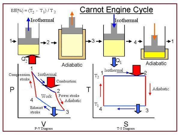
		The most efficient heat engine cycle is the Carnot cycle, consisting of two isothermal processes and two adiabatic processes (see Figure 08). The Carnot cycle can be thought of as the most efficient heat engine cycle allowed by physical laws. When the second law of thermodynamics states that not all the supplied heat in a heat engine can be used to do work, the Carnot efficiency sets the limiting value on the fraction of the heat which can be so used. In order to approach the Carnot efficiency, the processes involved in the heat engine cycle
Figure 07 Heat Engine [view large image]	Figure 08 Carnot Engine Cycle [view large image]	must be reversible and involve no change in entropy. This means that the Carnot cycle is an idealization, since no real engine processes are reversible and all real physical processes involve some increase in entropy.

			The p-V diagrams for the more realistic cases are shown in Figure 09, 10, and 11 for the gasoline, diesel, and steam engines respectively. While the gasoline and diesel engines operate at about 50% efficiency, the steam engine runs at only about 30%. A brief description of the processes can be found in each of the diagram.
Figure 09 Gasoline Engine [view large image]	Figure 10 Diesel Engine [view large image]	Figure 11 Steam Engine [view large image]

---

Connection to the Microscopic View

The branch of physics known as statistical mechanics attempts to related the macroscopic properties of an assembly of particles to the microscopic properties of the particles themselves. Statistical mechanics, as its name implies is not concerned with the actual motions or interactions of individual particles, but investigates instead their most probable behavior. The state of a system of particles is completely specified classically at a particular instant if the position r and velocity v of each of its constituent particles are known. The number of particles occupying an infinitesimal cell in the

Statistical mechanics - Definition

Statistical mechanics is the application of statistics, which includes mathematical tools for dealing with large populations, to the field of mechanics, which is concerned with the motion of particles or objects when subjected to a force. It provides a framework for relating the microscopic properties of individual atoms and molecules to the macroscopic or bulk properties of materials that can be observed in every day life, therefore explaining thermodynamics as a natural result of statistics and mechanics (classical and quantum). In particular, it can be used to calculate the thermodynamic properties of bulk materials from the spectroscopic data of individual molecules.

Contents [showhide]

1 Microscopic entropy, the Boltzmann factor and the partition function 2 Connection with thermodynamics 3 Variable particle number 4 Further development 5 Grand canonical ensemble 6 See also

Microscopic entropy, the Boltzmann factor and the partition function

At the heart of statistical mechanics lies Boltzmann's definition of entropy of a physical system:

The entropy of a macroscopic state is proportional to the logarithm of the number of microscopic states corresponding to it.

Boltzmann's proportionality constant is denoted k. See microcanonical ensemble. Let's introduce the standand β=1/kT.

From this definition it is possible to deduce the fact that, if a system is in contact with a heat bath, the probability of a microstate of energy E is proportional to

<math>\exp\left(-\beta E\right)<math>

where the temperature T arises from the fact that the system is in equilibrium with the heat bath (see canonical ensemble). This quantity is called the Boltzmann factor. The probabilities of the various microstates must add to one, and the normalization factor is the partition function:

<math>Z = \sum_i \exp\left(-\beta E_i\right)<math>

where <math>E_i<math> is the energy of the ith microstate of the system. The partition function is a measure of the number of states accessible to the system at a given temperature. See derivation of the partition function for a proof of Boltzmann's factor and the form of the partition function from first principles.

To sum up, the probability of finding a system at temperature T in a particular state with energy E_i is

<math>p_i = \frac{\exp(-\beta E_i)}{Z}<math>

Connection with thermodynamics

The partition function can be used to find the expected (average) value of any microscopic property of the system, which can then be related to macroscopic variables. For instance, the expected value of the microscopic energy E is interpreted as the microscopic definition of the thermodynamic variable internal energy (U)., and can be obtained by taking the derivative of the partition function with respect to the temperature. Indeed,

<math>\langle E\rangle={\sum_i E_i e^{-\beta E_i}\over Z}=-{dZ\over d\beta}/Z<math>

implies, together with the interpretation of <E> as U, the following microscopic definition of internal energy:

<math>U\colon = -{d\ln Z\over d \beta}.<math>

The entropy can be calculated by (see Shannon entropy)

<math>{S\over k} = - \sum_i p_i \ln p_i = \sum_i {e^{-\beta E_i}\over Z}(\beta E_i+\ln Z) = \ln Z + \beta U <math>

which implies that

<math>-\frac{\ln(Z)}{\beta} = U - TS = F<math>

is the Free energy of the system or in other words,

<math>Z=e^{-\beta F}\,<math>

Having microscopic expressions for the basic thermodynamic potentials U (internal energy), S (entropy) and F (free energy) is sufficient to derive expressions for other thermodynamic quantities. The basic strategy is as follows. There may be an intensive or extensive quantity that enters explicitly in the expression for the microscopic energy E_i, for instance magnetic field (intensive) or volume (extensive). Then, the conjugate thermodynamic variables are derivatives of the internal energy. For instance, the macroscopic magnetization (extensive) is the derivative of U with respect to the (intensive) magnetic field, and the pressure (intensive) is the derivative of U with respect to volume (extensive).

Variable particle number

That was the version for systems which don't allow an exchange of matter. Otherwise, if matter can be exchanged and particle number is conserved, we would have to introduce chemical potentials, μ_j, j=1,...,n and replace the partition function with

<math>Z = \sum_i \exp\left(\beta \left[\sum_{j=1}^n \mu_j N_{ij}-E_i\right ]\right)<math>

where N_ij is the number of j^th species particles in the i^th configuration. Sometimes, we also have other variables to add to the partition function, one corresponding to each conserved quantity. Most of them, however, can be safely interpreted as chemical potentials. In most condensed matter systems, things are nonrelativistic and mass is conserved. However, most condensed matter systems of interest also conserve particle number approximately (metastably) and the mass (nonrelativistically) is none other than the sum of the number of each type of particle times its mass. Mass is inversely related to density, which is the conjugate variable to pressure. For the rest of this article, we will ignore this complication and pretend chemical potentials don't matter. See grand canonical ensemble.

Further development

The treatment in this section assumes no exchange of matter (i.e. fixed mass and fixed particle numbers). However, the volume of the system is variable which means the density is also variable.

This probability can be used to find the average value, which corresponds to the macroscopic value, of any property, <math>J<math>, that depends on the energetic state of the system by using the formula:

<math> \langle J \rangle = \sum_i p_i J_i = \sum_i J_i \frac{\exp(-\beta E_i)}{Z}<math>

where <math><math> is the average value of property <math>J<math>. This equation can be applied to the internal energy, <math>U<math>:

<math>U = \sum_i E_i \frac{\exp(\beta E_i)}{Z}<math>

Subsequently, these equations can be combined with known thermodynamic relationships between <math>U<math> and V to arrive at an expression for pressure in terms of only temperature, volume and the partition function. Similar relationships in terms of the partition function can be derived for other thermodynamic properties as shown in the following table.

Helmholtz free energy:	<math>F = - {\ln Z\over \beta}<math>
Internal energy:	<math>U = -\left( \frac{\partial\ln Z}{\partial\beta} \right)_{N,V}<math>
Pressure:	<math>P = -\left({\partial F\over \partial V}\right)_{N,T}= {1\over \beta} \left( \frac{\partial \ln Z}{\partial V} \right)_{N,T}<math>
Entropy:	<math>S = k (\ln Z + \beta U)\,<math>
Gibbs free energy:	<math>G = F+PV=-{\ln Z\over \beta} + {V\over \beta} \left( \frac{\partial \ln Z}{\partial V}\right)_{N,T}<math>
Enthalpy:	<math>H = U + PV\,<math>
Constant Volume Heat capacity:	<math>C_V = \left( \frac{\partial U}{\partial T} \right)_{N,V}<math>
Constant Pressure Heat capacity:	<math>C_P = \left( \frac{\partial U}{\partial T} \right)_{N,P}<math>
Chemical potential:	<math>\mu_i = -{1\over \beta} \left( \frac{\partial \ln Z}{\partial N_i} \right)_{T,V,N}<math>

The last entry needs clarification. We are NOT working with a grand canonical ensemble here.

It is often useful to consider the energy of a given molecule to be distributed among a number of modes. For example, translational energy refers to that portion of energy associated with the motion of the center of mass of the molecule. Configurational energy refers to that portion of energy associated with the various attractive and repulsive forces between molecules in a system. The other modes are all considered to be internal to each molecule. They include rotational, vibrational, electronic and nuclear modes. If we assume that each mode is independent (a very questionable assumption!!!!!) the total energy can be expressed as the sum of each of the components:

<math>E = E_t + E_c + E_n + E_e + E_r + E_v\,<math>

Where the subscripts t, c, n, e, r, and v correspond to translational, configurational, nuclear, electronic, rotational and vibrational modes, respectively. The relationship in this equation can be substituted into the very first equation to give:

<math>Z = \sum_i \exp\left(-\beta(E_{ti} + E_{ci} + E_{ni} + E_{ei} + E_{ri} + E_{vi})\right)<math>

<math>= \sum_i

\exp\left(-\beta E_{ti}\right) \exp\left(-\beta E_{ci}\right) \exp\left(-\beta E_{ni}\right) \exp\left(-\beta E_{ei}\right) \exp\left(-\beta E_{ri}\right) \exp\left(-\beta E_{vi}\right)<math>

<math>= Z_t Z_c Z_n Z_e Z_r Z_v\,<math>

Thus a partition function can be defined for each mode. Simple expressions have been derived relating each of the various modes to various measurable molecular properties, such as the characteristic rotational or vibrational frequencies.

Expressions for the various molecular partition functions are shown in the following table.

Nuclear	<math>Z_n = 1 \qquad (T < 10^8 K)<math>
Electronic	<math>Z_e = W_0 \exp(kT D_e + W_1 \exp(-\theta_{e1}/T) + \cdots)<math>
vibrational	<math>Z_v = \prod_j \frac{\exp(-\theta_{vj} / 2T)}{1 - \exp(-\theta_{vj} / T)}<math>
rotational (linear)	<math>Z_r = \frac{T}{\sigma} \theta_r<math>
rotational (non-linear)	<math>Z_r = \frac{1}{\sigma}\sqrt{\frac{{\pi}T^3}{\theta_A \theta_B \theta_C}}<math>
Translational	<math>Z_t = \frac{(2 \pi mkT)^{3/2}}{h^3}<math>
Configurational (ideal gas)	<math>Z_c = V\,<math>

These equations can be combined with those in the first table to determine the contribution of a particular energy mode to a thermodynamic property. For example the "rotational pressure" could be determined in this manner. The total pressure could be found by summing the pressure contributions from all of the individual modes, ie:

<math>P = P_t + P_c + P_n + P_e + P_r + P_v\,<math>

Grand canonical ensemble

Let's rework everything using a grand canonical ensemble this time. The volume is left fixed and does not figure in at all in this treatment. As before, j is the index for those particles of species j and i is the index for microstate i:

<math>U = \sum_i E_i \frac{\exp(-\beta (E_i-\sum_j \mu_j N_{ij}))}{Z}<math>

<math>N_j = \sum_i N_{ij} \frac{\exp(-\beta (E_i-\sum_i \mu_j N_{ij}))}{Z}<math>

Gibbs free energy:	<math>G = - {\ln Z\over \beta}<math>
Internal energy:	<math>U = -\left( \frac{\partial\ln Z}{\partial\beta} \right)_{\mu}+\sum_i{\mu_i\over\beta}\left({\partial \ln Z\over \partial \mu_i}\right )_{\beta}<math>
Particle number:	<math>N_i={1\over\beta}\left({\partial \ln Z\over \partial \mu_i}\right)_\beta<math>
Entropy:	<math>S = k (\ln Z + \beta U- \beta \sum_i \mu_i N_i)\,<math>
Helmholtz free energy:	<math>F = G+\sum_i \mu_i N_i=-{\ln Z\over \beta} +\sum_i{\mu_i\over \beta} \left( \frac{\partial \ln Z}{\partial \mu_i}\right)_{\beta}<math>

http://www.wordiq.com/definition/Statistical_mechanics

Héctor A.Chacón C.

Statistical Mechanics Entropy Revisited

In the study of heat, and of thermodynamics in general, there was no need to know the microscopic nature of the substance which was being heated or cooled and so on. Instead, we reasoned using general principles such as temperature, work, and energy conservation and explained a number of important phenomenon. We then introduced the idea of entropy, which is needed for explaining the physically observed irreversibility of the world around us. The Second Law of Thermodynamics was then shown to imply a number of new results, including the fact that there can never be a perpetual motion machine. The idea of energy is well understood from mechanics. To explain thermodynamics the new and profound idea of entropy had to be invented. It is the idea of entropy that is central and unique to the study of heat and thermodynamics, and the branch of physics called statistical mechanics has resulted from the attempt to understand entropy from a microscopic point of view. Recall from (9.41) we have a microscopic definition of entropy given by 

The microscopic definition unavoidably led to assumptions as to what matter is made out of, namely what is the microscopic composition of matter. For example, in applying the equation for entropy to the case of an ideal gas, we had to take into account the microscopic nature of the gas, in particular, that it is made out of an enormous collection of microscopic objects that we identified with atoms. The entire field of statistical mechanics was founded by Boltzmann in the late nineteenth century. As a historical aside, it is worth recording that it was in order to understand the concept of entropy from a microscopic point of view, that Boltzmann had postulated the existence of atoms well before their discovery in the twentieth century. In sum, the challenge posed by thermodynamics was the following: how can we reconcile ideas such as temperature, entropy and so on with the ideas of (Newtonian) mechanics? In particular, if any sample of matter that we observe in daily life is made out of an inordinately large number of atoms, approximately , how can we apply the laws of mechanics to this large collection of particles? Clearly, it is hopeless to try and describe how every single particle is moving, as this would involve specifying, at each instant, number of positions and velocities. So what is the way out of this impasse?

Classical Statistical Mechanics

We know for a fact that all matter is composed out of small particles called atoms. Statistical mechanics is that branch of physics which explains the thermodynamic properties of nature starting from a microscopic point of view. In particular, we will attempt to apply classical mechanics to a large collection of particles, and in this way derive all the results of thermodynamics. We know that classical (Newtonian) mechanics cannot explain why atoms even exist, let alone explain its properties for which quantum mechanics is necessary. So can we, at all, classically analyze a large collection of atoms before understanding quantum mechanics? The answer, surprisingly enough, is yes. The reason is the following. In studying statistical mechanics, we will be concerned with the object's bulk (macroscopic) properties such as temperature, energy and so on. These properties result mainly from the interaction of atoms (and molecules) with each other. Recall atoms are electrically neutral, and are composed of a positively charged nucleus and negatively charged electrons which are distributed outside the nucleus. Let there be two atoms at positions and . The distance between them is then given by ; the so called Lennard-Jones potential results from the quantum mechanical interaction of the charges and angular momentum that is carried by the atoms. The potential due to a typical atom or molecule is given by

(10.1)

where is a constant which depends on charge, and is the Lennard-Jones (LJ) radius, and is shown in Figure 10.1. Note that there is a minimum value in the inter-atomic potential at a distance of from the atom.

Figure 10.1: Lennard-Jones Potential

As long as the atoms are moving slowly, and are farther away from each other than distance , they can be treated as hard spheres of radius that behave as classical particles. For typical atoms and molecules the LJ-radius is around 3 to 5A (A= Angstrom =). For example, for the argon atom, the LJ radius is 3.5A, and is 5A for a large molecule such as propane. However, in some cases the LJ radius is not suitable for determining the effective classical size of an atom. For example the molecule has an LJ radius of 0.7A, and is too small a distance to be taken as the classical radius of the molecule. As long as the object being analyzed is at temperatures and densities that are not very high or very low, the atoms are not squeezed together closer than the distance of the LJ radius, and we can treat the atoms as classical billiard balls. However at very low temperatures and high densities, this is not true and the classical analysis needs to replaced by quantum mechanics. At very high temperatures, the inner structure of the atoms, composed as it is out of a nucleus and electrons, needs to be taken into account, and requires an analysis which goes beyond classical mechanics.

Ensembles

We can now return to the problem at hand, namely that we have a collection of number of classical particles, thought of as hard spheres of radius , having mass , and at temperature . We would like to derive all the thermodynamic properties of the object in question starting from Newtonian mechanics. For the sake of concreteness, let us consider an ideal gas at temperature , confined in a container of volume , and let us further suppose that the gas is in equilibrium. By the gas being ideal, we mean that all the interactions of the particles which compose the gas can be ignored. The energy of the gas hence consists entirely of kinetic energy; let the three-dimensional velocity of the -th particle be denoted by . Since there are particles, the total kinetic energy of the gas is simply the sum of the kinetic energies of the individual particles (atoms). Hence the energy of the gas is given by the following

(10.2)

Recall that by equilibrium we mean that the gas has attained a state of maximum entropy, or equivalently, that there are no more changes of temperature and other state variable taking place. By the statement that the gas is at temperature , we mean that the gas in question is in contact with a heat bath which is at a temperature . The very fact that we have introduced the physical idea of temperature already implies that the gas is not an isolated system, but rather is part of a larger system which includes the heat bath and the object at a given temperature.

Figure 10.2: Gas in contact with a heat bath

How do we describe a gas, shown in Figure 10.2, composed out of particles, occupying a volume and at temperature ? There are simply too many particles to keep track of. To provide a mechanical description of the gas, we need to know the exact position and velocity of each and every particle, and which in general, is called a microstate of the system. A description of the microstate of any large object, containing about Avogardo's number of atoms, is in practice too difficult. And even more importantly, there is no need since the questions asked in thermodynamics do not refer to any single atom composing the gas, but rather, refer to the properties of the gas taken as a whole, called the bulk properties of the gas. We now make a major conceptual leap. We postulate that having a gas at a temperature means that the gas is not in a definite (mechanical) microstate state. Instead, all the various (mechanical) microstates states of the gas are now taken to occur with a certain probability. Hence, the description of the gas by its microstates, that is, by the detailed knowledge of the position and momentum of each and every atom of the gas, is replaced by an ensemble of microstates. An ensemble is a collection of all the possible microstates of the gas. The ensemble is called a microcanonical, canonical or grand canonical depending on the way that probabilities are assigned for the occurrence of the various microstate . We will return to this question is some detail in Section . Since we know nothing of the microstates of the gas, the most consistent manner of assigning a probability of occurrence for the various allowed microstates is to assume that all the microstates of the gas are equally likely; this is how a microcanonical ensemble is defined. Our ignorance of the microstates is consequently given a complete expression in the microcanonical ensemble which is defined as follows. Given the parameters such as energy, volume and so on that specify the macroscopic properties of the gas, in the microcanonical ensemble all the microstates of the gas are equally likely. One should note that the idea of ensemble reflects our ignorance as to what is the microstate of the gas. The gas is inherently not in a probabilistic state, but rather it is our inability to determine its state which has led us to the ideas of probability, and to the idea of classical uncertainty. In quantum mechanics we will encounter uncertainty which is not a function of our ignorance, but rather, is an intrinsic property of nature. In the language of probability theory, the positions and velocities are all considered to be continuous random variables. In other words, the velocity of the particle has no definite value, but rather, its probability of occurrence is determined by the ensemble that describes it. We will denote by brackets the average value of a random variable. Hence, the average value of the kinetic energy of the th particle is denoted by . In Section 4 we will examine more closely how to calculate the average value of various physical quantities including kinetic energy.

Kinetic Theory of Gases

As the first application of the idea of ensembles, we discuss the kinetic theory of gases. This theory is applicable to a dilute gas that, to a good degree of accuracy, can be considered to be an ideal gas. Recall every atom of the gas is considered to be a free classical particle with mass and having a random velocity . We will use the term atom and particle interchangeably.

Pressure

From the atomic point of view, how does pressure arise? Even before going into the detailed mechanism, we expect that pressure should be a macroscopic manifestation of microscopic motion. Consider a frictionless piston, which has an area , contains a gas in some volume and with total number of atoms given by . The piston is in equilibrium with the gas at some temperature . Outside the piston is a perfect vacuum.

Figure 10.3: Gas Inside the Piston and Vacuum Outside

The atoms of the gas are constantly bombarding the piston and this will cause a force to be exerted on the piston, and to keep the piston in place (stationary) we need to counter this force. Consider for an atom traveling straight towards the piston with velocity ; we will show later the case of the atom moving with arbitrary velocity gives the same result. The particle hits the piston and bounces back. We assume that the collision is elastic in that the energy of the atom is the same before and after bouncing off the piston. The assumption of the collision being elastic means that the atom does not lose any of its energy to the piston. This is reasonable, since if it lost energy to the piston, the piston would heat up; and once the piston reached equilibrium with the gas, the assumption of collisions being elastic would be correct. As shown in Figure 10.4, for a wall placed along the -axis, an elastic collision leads to a velocity . Hence, for simplicity we consider only the special case of . Let the velocity of the atom after the collision be . Since the atom possesses only kinetic energy, we have from energy conservation

			(10.3)
			(10.4)

Figure 10.4: Diagram v to -v

Figure 10.5: Diagram v to -v

In other words, in colliding off the piston, the particle's velocity changed from to , and hence the momentum imparted to the piston is

(10.5)

In time , how many atoms will bounce off the piston? All the atoms with velocity can reach the piston in time if they are at a distance less than from the piston. Consequently, all the atoms in a volume of size will bounce off the piston. Hence, since the density (particles per unit volume) is , in time the momentum imparted to the piston is

			(10.6)
			(10.7)

Since the force on the piston is nothing but the rate at which momentum changes on the piston due to collisions of the gas atoms, we have

			(10.8)
			(10.9)

Recall pressure is defined to be force per unit area, and hence the pressure on the piston due to the gas is

			(10.10)
			(10.11)
			(10.12)

From the ensemble point of view, the velocity of the atom is a random variable, and what the piston really experiences is the average value over all possible velocities that the atoms has as it bounces off the piston. Hence, denoting as usual average values by , we have

(10.13)

The reason we have dropped the factor of in going from (10.12) to (10.13) is that we need to perform the average over only those particles which are heading towards the piston and not away from it. Since we are taking the average value of , we are over-counting by a factor of since we are also including the particles moving away from the piston. Recall we had considered a very special set of velocities, namely, those heading straight for the piston, and hence with . In general, the velocity of an arbitrary atom has the form . Since all directions for the gas are equivalent, we have

			(10.14)
			(10.15)

We finally have, from eq.(10.13), the following

(10.16)

The total energy, of the gas is solely composed of kinetic energy. Hence we have

(10.17)

From (10.13) and (10.15) and (10.17) we have

(10.18)

Temperature

We have so far been able to define both the pressure and energy of the gas from the atomic point of view. We now need to define temperature. Consider two gases in a cylinder separated by a frictionless piston. When the piston reaches equilibrium there is no further change in the system. We hence conclude that the temperature of both of the gases must be the same, since the very definition of temperature is that there will be heat flows, and consequently, no equilibrium, unless and until the temperatures of the two gases becomes equal.

Figure 10.6: Piston Separating out Two Gases

We now examine the conditions under which there will be equilibrium. Let us label the gas on the left of the cylinder as and that on the right as . For equilibrium, the pressure exerted by both the gases on the piston must be equal. Hence, from (10.16) we have

(10.19)

Are the densities of the two gases the same on two sides of the piston, that is equal to ? The answer is yes, although to prove this is quite difficult. The intuitive proof that the two densities are equal is that if there was a difference in the densities, there would be a net ``osmotic'' pressure on the piston forcing it to move, and consequently the system would not be in equilibrium. Hence, in equilibrium, we have

(10.20)

and from (10.19) we obtain

(10.21)

We see that the equation above is simply a statement that the average kinetic of the atoms in two gases which are in equilibrium is the same. Hence temperature is defined to be proportional to the average kinetic energy of a single atom of the gas. Fixing the constant of proportionality to be the Boltzmann constant we finally arrive at the following definition of temperature .

(10.22)

Temperature is a measure of how fast, on the average, that the atoms of a gas are moving. At room temperature eV. The faster the atoms move, the hotter the temperature. The sensation of burning that we have on putting our hands into, say a fire, is because fast moving atoms from the fire impart high amounts of kinetic energy to our hands, causing atoms in our hand to move very fast and result in the sensation of burning. Hence, from eqns.(10.2) and (10.22)we have

			(10.23)
			(10.24)

Combining our results, from (10.16) and (10.22) we finally obtain the ideal gas law

(10.25)

The result above has the remarkable implication that no matter what the gas is composed of, for example, be it nitrogen, helium and so on, equal volumes of the various gases at the same pressure and temperature have the same number N of atoms. Note this result follows directly from Newton's Laws as is seen by the derivation given. This remarkable property of the ideal gas led Avoagardo to postulate that one molar volume of any gas will have the same number of atoms, given by Avagardo's number .

http://srikant.org/core/node11.html

Héctor A. Chacón C.