lunes, 15 de febrero de 2010

Introducción

    Como muchas disciplinas, la termodinámica surge de los procedimientos empíricos que llevaron a la construcción de elementos que terminaron siendo muy útiles para el desarrollo de la vida del hombre.
Creemos que la termodinámica es un caso muy especial debido a que sus inicios se pierden en la noche de los tiempos mientras que en la actualidad los estudios sobre el perfeccionamiento de las máquinas térmicas siguen siendo de especial importancia, mas aun si tomamos en cuenta la importancia que revisten temas de tanta actualidad como la contaminación.

El origen fué sin lugar a dudas la curiosidad que despertara el movimiento producido por la energía del vapor de agua.
Su desarrollo fué tomando como objetivo principal el perfeccionamiento de las tecnologias aplicadas con el fin de hacer mas facil la vida del hombre, reemplazando el trabajo manual por la máquina que facilitaba su realización y lograba mayor rapidez, estos avances que gravitaban directamente en la economía, por ello el inicio se encuentra en el bombeo de aguas del interior de las minas y el transporte.
Mas tarde se intensificaron los esfuerzos por lograr el máximo de rendimiento lo que llevó a la necesidad de lograr un conocimiento profundo y acabado de las leyes y principios que regian las operaciones realizadas con el vapor.

    El campo de la termodinámica y su fuente primitiva de recursos se amplía en la medida en que se incorporan nuevas áreas como las referentes a los motores de combustión interna y ultimamente los cohetes. La construcción de grandes calderas para producir enormes cantidades de trabajo marca tambien la actualidad de la importancia del binomio máquinas térmicas-termodinámica.

En resumen: en el comienzo se partió del uso de las propiedades del vapor para succionar agua de las minas, con rendimientos insignificantes, hoy se trata de lograr las máximas potencias con un mínimo de contaminación y un máximo de economía.
Para realizar una somera descripción del avance de la termodinámica a través de los tiempos la comenzamos identificando con las primitivas máquinas térmicas y dividimos su descripción en tres etapas, primero la que dimos en llamar empírica, la seguna la tecnológica y la tercera la científica.

I.- La etapa empírica

    Los orígenes de la termodinámica nacen de la pura experiencia y de hallazgos casuales que fueron perfeccionándose con el paso del tiempo.

Algunas de las máquinas térmicas que se construyeron en la antigüedad fueron tomadas como mera curiosidad de laboratorio, otros se diseñaron con el fin de trabajar en propósitos eminentemente prácticos. En tiempos del del nacimiento de Cristo existian algunos modelos de máquinas térmicas, entendidas en esa época como instrumentos para la creación de movimientos autónomos, sin la participación de la tracción a sangre.

El ingenio más conocidos por las crónicas de la época es la eolipila de Herón que usaba la reacción producida por el vapor al salir por un orificio para lograr un movimiento. Esta máquina es la primera aplicacióndel principio que usan actualmente las llamadas turbinas de reacción.

La historia cuenta que en 1629 Giovanni Branca diseñó una máquina capaz de realizar un movimiento en base al impulso que producía sobre una rueda el vapor que salía por un caño. No se sabe a ciencia cierta si la máquina de Branca se construyó, pero, es claro que es el primer intento de construcción de las que hoy se llaman turbinas de acción.

La mayor aplicación de las posibilidades de la máquina como reemplazante de la tracción a sangre consistía en la elevación de agua desde el fondo de las minas. Por ello la primera aplicación del trabajo mediante la fuerza del vapor cristaliza en la llamada máquina de fuego de Savery.

La máquina de Savery consistía en un cilindro conectado mediante una cañería a la fuente de agua que se deseaba bombear, el cilindro se llenaba de vapor de agua, se cerraba la llave de ingreso y luego se enfriaba, cuando el vapor se condensaba se producía un vacío que permitía el ascenso del agua.

II.- La etapa tecnológica.
     Según lo dicho la bomba de Savery no contenía elementos móviles, excepto las válvulas de accionamiento manual, funcionaba haciendo el vacío, de la misma manera en que ahora lo hacen las bombas aspirantes, por ello la altura de elevación del agua era muy poca ya que con un vacío perfecto se llegaría a lograr una columna de agua de 10.33 metros, pero, la tecnología de esa época no era adecuada para el logro de vacios elevados.

El primer aparato elemento que podriamos considerar como una máquina propiamente dicha, por poseer partes móviles, es la conocida como máquina de vapor de Thomas Newcomen construída en 1712. La innovación consistió en la utilización del vacío del cilindro para mover un pistón que a su vez proveía movimiento a un brazo de palanca que actuaba sobre una bomba convencional de las llamadas aspirante-impelente.

Podemos afirmar que es la primera máquna alternativa de mla que se tiene conocimiento y que con ella comienza la historia de las máquinas térmicas.

Las dimensiones del cilindro, órgano principal para la creación del movimien-to, eran: 53,3 cm de diámetro y 2,4 metros de altura, producía 12 carreras por minuto y elevaba 189 litros de agua desde una profundidad de 47,5 metros.
El principal progreso que se incorpora con la máquina de Newcomen consis-te en que la producción de un movimiento oscilatorio habilita el uso de la máquina para otros servicios que requieran movimiento alternativo, es decir, de vaivén.

En esa época no existian métodos que permitieran medir la potencia desarrollada por las máquinas ni unidades que permitieran la comparación de su rendi-miento, no obstante, los datos siguientes dan una idea del trabajo realizado por una máquina que funcionó en una mina en Francia, contaba con un cilindro de 76 cm de diámetro y 2,7 metros de altura, con ella se pudo completar en 48 horas una labor de desagote que previamente había requerido una semana con el traba-jo de 50 hombres y 20 caballos operando en turnos durante las 24 horas del día.

La máquina de Newcomen fué perfeccionada por un ingeniero inglés llamado Johon Smeaton (1742-1792). Un detalle de la potencia lograda lo podemos ver en el trabajo encargado por Catalina II de Rusia quien solicitó bombear agua a los di-ques secos del fuerte de Kronstadt. Esta tarea demoraba un año usando molinos de viento de 100 metros de altura, la máquina de Smeaton demoró solamente dos semanas. Se debe destacar que el perfeccionamiento consistió en la optimización de los mecanismos, cierres de válvulas, etc.

El análisis de las magnitudes que entran en juego en el funcionamiento de la máquina de vapor y su cuantificación fué introducido por James Watt (1736-1819).
Watt se propuso estudiar la magnitud del calor puesto en juego en el funcio-namiento de la máquina, esto permitiría estudiar su rendimiento.

El mayor obstáculo que encontró Watt fué el desconocimiento de los valores de las constantes físicas involucradas en el proceso, a raiz de ello debió realizar un proceso de mediciones para contar con datos confiables.
Sus mediciones experimentales le permitieron verificar que la máquina de Newcomen solo usaba un 33% del vapor consumido para realizar el trabajo útil.

Los aportes de Watt son muchos, todos ellos apuntaron al logro de un mayor rendimiento, inventó el prensaestopa que actua manteniendo la presión mientras se mueve el bástago del pistón, introdujo la bomba de vacío para incrementar el rendimiento en el escape, ensayó un mecanismo que convirtiera el movimiento alternativo en rotacional, en 1782 patentó la máquina de doble efecto (el vapor empuja en ambas carreras del pistón), ideó válvulas de movimiento vertical que permitian mantener la presión de la caldera mediante la fuerza de un resorte com-primido. Creó el manómetro para medir la presión del vapor y un indicador que po-día dibujar la evolución presión-volumen del vapor en el cilindro a lo largo de un ciclo.
Con el objetivo de establecer una unidad adecuada para la medición de la potencia, realizó experiencias para definir el llamado caballo de fuerza. Determinó que un caballo podía desarrollar una potencia equivalente a levantar 76 kg hasta una altura de 1 metro en un segundo, siguiendo con este ritmo durante cierto tiempo, este valor se usa actualmente y se lo llama caballo de fuerza inglés.

Un detalle importante de las calderas de Watt es que trabajaban a muy baja presión, 0,3 a 0,4 kg/cm2.
Los progresos tecnológicos aportados por Watt llevaron la tecnología de la máquina de vapor a un refinamiento considerable. Se había avanzado en seguri-dad merced a la incorporación de válvulas, ya se contaba con unidades que daban cuenta de la potencia y el rendimiento, los mecanismos fueron elaborados con los mas recientes avances de la tecnología mecánica. Lo único que no entró en la consideración de Watt fué la posibilidad de usar calderas de mayor presión, su objetivo principal era la seguridad, y desde el punto de vista económico no reque-ría perfeccionamiento, sus máquinas eran muy apreciadas y se vendian bien.

Después de Watt se consiguieron considerables avances en la utilización de calderas de muy alta presión, esta incorporación incrementó el rendimiento y, lo mas importante, favoreció el uso de calderas de menor tamaño que realizaban mayor trabajo que las grandes, además de mejorar el rendimiento del vapor las preparó para adaptarlas para su instalación en medios de transporte.
En agosto de 1807 Robert Fulton puso en funcionamiento el primer barco de vapor de éxito comercial, el Clermont, el mérito de Fulton consiste en la instalación y puesta en marcha de una máquina de vapor a bordo, no realizó innovaciones sobre la máquina en sí. Este barco cumplió un servicio fluvial navegando en el río Hudson.

En el año 1819 el buque de vapor Savannah, de bandera norteamericana realiza el primer viaje transatlántico, ayudado por un velamen. El Britania fué el primer barco de vapor inglés, entró en servicio en 1840, desplazaba 1150 toneladas y contaba con una máquina de 740 caballos de fuerza, alimentada por cuatro calderas de 0.6 kg/cm cuadrado, desarrollando una velocidad de 14 km/h.

George Stephenson (1781-1848) fué el primero que logró instalar una máquina de vapor sobre un vehículo terrestre dando inicio a la era del ferrocarril.

En el año 1814 Stephenson logró arrastrar una carga de treinta toneladas por una pendiente de 1 en 450 a sis km por hora.
En 1829 la locomotora llamada Rocket recorrió 19 km en 53 minutos lo que fué un record para la época.

III.- Etapa científica.

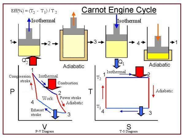
    Sadi Carnot (1796-1832) es el fundador de la termodinámica como disciplina teórica, escribió su trabajo cumbre a los 23 años. Este escrito estuvo desconocido durante 25 años hasta que el físico Lord Kelvin redescubriera la importancia de las propuestas contenidas en él.

Llamó la atención de Carnot el hecho de que no existieran teorias que ava-laran la propuestas utilizadas en el diseño de las máquinas de vapor y que todo ello dependira de procedimientos enteramente empíricos. Para resolver la cuestión propuso que se estudiara todo el procedimiento desde el punto de vista mas gene-ral, sin hacer referencia a un motor, máquina o fluido en especial.

Las bases de las propuestas de Carnot se pueden resumir haciendo notar que fué quien desarrolló el concepto de proceso cíclico y que el trabajo se produ-cía enteramente "dejando caer" calor desde una fuente de alta temperatura hasta un depósito a baja temperatura. También introdujo el concepto de máquina reversible.

El principio de Carnot establece que la máxima cantidad de trabajo que puede ser producido por una máquina térmica que trabaja entre una fuente a alta temperatura y un depósito a temperatura menor, es el trabajo producido por una máquina reversible que opere entre esas dos temperaturas. Por ello demostró que ninguna máquina podía ser mas eficiente que una máquina reversible.
A pesar que estas ideas fueron expresadas tomando como base la teoría del calórico, resultaron válidas. Posteriormente Clausius y Kelvin, fundadores de la termodinámica teórica, ubicaron el principio de Carnot dentro de una rigurosa teo-ría científica estableciendo un nuevo concepto, el segundo principio de la termodinámica.

Carnot también establece que el rendimiento de cualquier máquina térmica depende de la diferencia entre temperatura de la fuente mas caliente y la fría. Las altas temperaturas del vapor presuponen muy altas presiones y la expansión del vapor a bajas temperaturas producen grandes volúmenes de expansión. Esto producía una cota en el rendimiento y la posibilidad de construcción de máquinas de vapor.

En esta época todavía tenía vigencia la teoría del calórico, no obstante ya estaba germinando la idea de que esa hipótesis no era la adecuada, en el marco de las sociedades científicas las discusiones eran acaloradas.
James Prescot Joule (1818-1889) se convenció rapidamente de que el trabajo y el calor eran diferentes manifestaciones de una misma cosa. Su expe-riencia mas recordada es aquella en que logra medir la equivalencia entre el traba-jo mecánico y la cantidad de calor. Joule se valió para esta experiencia de un sis-tema de hélices que agitaban el agua por un movimiento producido por una serie de contrapesos que permitian medir la energía mecánica puesta en juego.
A partir de las investigaciones de Joule se comenzó a debilitar la teoría del calórico, en especial en base a los trabajos de Lord Kelvin quien junto a Clausius terminaron de establecer las bases teóricas de la termodinámica como disciplina independiente. En el año 1850 Clausius dscubrió la existencia de la entropía y enunció el segundo principio:

Es imposible que una máquina térmica que actúa por sí sola sin recibir ayuda de ningún agente externo, transporte calor de un cuerpo a otro que está a mayor temperatura.

En 1851 Lord Kelvin publicó un trabajo en el que compatibilizaba los estudios de Carnot, basados en el calórico, con las conclusiones de Joule, el calor es una forma de energía, compartió las investigaciones de Clausius y reclamó para sí el postulado del primer principio que enunciaba así:

Es imposible obtener, por medio de agentes materiales inanimados, efectos mecánicos de cualquier porción de materia enfriándola a una temperatura inferior a la de los objetos que la rodean.
Lord Kelvin también estableció un principio que actualmente se conoce como el primer principio de la termodinámica. Y junto a Clausius derrotaron la teoría del calórico.
Situación Actual

     Hoy se ha llegado a uninteresante perfeccionamiento de las máquinas térmicas, sobre una teoría basada en las investigaciones de Clausius, Kelvin y Carnot, cuyos principios están todavía en vigencia, la variedad de máquinas térmicas va desde las grandes calderas de las centrales nucleares hasta los motores cohete que impulsan los satélites artificiales, pasando por el motor de explosión, las turbinas de gas, las turbinas de vapor y los motores de retropropulsión. Por otra parte la termodinámica como ciencia actua dentro de otras disciplinas como la química, la biología, etc.

Conclusión

     El desarrollo de la termodinámica tiene un origen empírico como muchas de las partes de la tecnología.
Una de las curiosidades en la aplicación temprana de efectos del vapor en la etapa que dimos en llamar empírica y que a lo largo de su desarrollo cambiara su origen en varias hipótesis, flogisto, calórico y finalmente energía.
Con Watt se logra el perfeccionamiento en la tecnología, se comprenden los principios básicos de la misma y se aislan las variables que intervienen en el fun-cionamiento de la máquina, la introducción de la unidad para medir la potencia conduce al manejo de criterios de comparación.

Despues de Watt comienza el desarrollo de las máquinas móviles con las realizaciones de Robert Fulton y George Stephenson.
Tambien es importante marcar como las teorias de Carnot tienen aún validez en su forma original apesar de haber estado fundamentadas en una hipótesis erro-nea, la del calórico. Carnot introduce tres conceptos fundamentales:
El concepto de ciclo o máquina cíclica.

La relación entre la "caida del calor de una fuente caliente a otra mas fría y su relación con el trabajo.
El concepto de máquina reversible de rendimiento máximo.
Gracias a Clausius y Kelvin se convierte a la termodinámica en una ciencia independiente de alto contenido teórico y matemático, lo que logra entender los fenómenos que se desarrollaban y fundamentar progresos tecnológicos.


Bibliografía de referencia
Motores térmicos e hidráulicos
Rosich
Ergon
Termodinámica Técnica
Estrada
Editorial Alsina.
Maquinas Térmicas
Sandfort
Eudeba
A TextBook on Heat
Barton
Longsman
Heat
Mitton
Dent and sons
Las palabras clave se refieren a los precursores de esta ciencia: Herón, Savery, Newcomen, Fulton, Stephenson, Sadi Carnot, Clausius, Lord Kelvin, Joule, Watt.


Bárbara Scarlett Betancourt Morales


domingo, 14 de febrero de 2010

Equilibrium by Entropy Maximisation

Thermodynamics and Statistical Mechanics


P. Attard

Preface
Thermodynamics deals with the general principles and laws that govern the behaviour of matter and with the relationships between material properties. The origins of these laws and quantitative values for the properties are provided by statistical mechanics, which analyses the interaction of molecules and provides a detailed description of their behaviour. This book presents a unified account of equilibrium thermodynamics and statistical mechanics using entropy and its maximisation.
A physical explanation of entropy based upon the laws of probability is introduced. The equivalence of entropy and probability that results represents a return to the original viewpoint of Boltzmann, and it serves to demonstrate the fundamental unity of thermodynamics and statistical mechanics, a point that has become obscured over the years. The fact that entropy and probability are objective consequences of the mechanics of molecular motion provides a physical basis and a coherent conceptual framework for the two disciplines. The free energy and the other thermodynamic potentials of thermodynamics are shown simply to be the total entropy of a subsystem and reservoir; their minimisation at equilibrium is nothing but the maximum of the entropy mandated by the second law of thermodynamics and is manifest in the peaked probability distributions of statistical mechanics. A straightforward extension to nonequilibrium states by the introduction of appropriate constraints allows the description of fluctuations and the approach to equilibrium, and clarifies the physical basis of the equilibrium state. Although this book takes a different route to other texts, it shares with them the common destination of explaining material properties in terms of molecular motion. The final formulae and interrelationships are the same, although new interpretations and derivations are offered in places. The reasons for taking a detour on some of the less-travelled paths of thermodynamics and statistical mechanics are to view the vista from a different perspective, and to seek a fresh interpretation and a renewed appreciation of well-tried and familiar results. In some cases this reveals a shorter path to known solutions, and in others the journey leads to the frontiers of the disciplines. The book is basic in the sense that it begins at the beginning and is entirely self-contained. It is also comprehensive and contains an account of all of the modern techniques that have proven useful in modern equilibrium, classical statistical mechanics. The aim has been to make the subject matter broadly accessible to advanced students, whilst at the same time providing a reference text for graduate scholars and research scientists active in the field. The later chapters deal with more advanced applications, and while their details may be followed step-by-step, it may require a certain experience and sophistication to appreciate their point and utility. The emphasis throughout is on fundamental principles and upon the relationship between various approaches. Despite this, a deal of space is devoted to applications, approximations, and computational algorithms; thermodynamics and statistical mechanics were in the final analysis developed to describe the real world, and while their generality and universality are intellectually satisfying, it is their practical application that is their ultimate justification. For this reason a certain pragmatism that seeks to convince by physical explanation rather than to convict by mathematical sophistry pervades the text; after all, one person's rigor is another's mortis. The first four chapters of the book comprise statistical thermodynamics. This takes the existence of weighted states as axiomatic, and from certain physically motivated definitions, it deduces the familiar thermodynamic relationships, free energies, and probability distributions. It is in this section that the formalism that relates each of these to entropy is introduced. The remainder of the book comprises statistical mechanics, which in the first place identifies the states as molecular configurations, and shows the common case in which these have equal weight, and then goes on to derive the material thermodynamic properties in terms of the molecular ones. In successive chapters the partition function, particle distribution functions, and system averages, as well as a number of applications, approximation schemes, computational approaches, and simulation methodologies, are discussed. Appended is a discussion of the nature of probability. The paths of thermodynamics and statistical mechanics are well-travelled and there is an extensive primary and secondary literature on various aspects of the subject. Whilst very many of the results presented in this book may be found elsewhere, the presentation and interpretation offered here represent a sufficiently distinctive exposition to warrant publication. The debt to the existing literature is only partially reflected in the list of references; these in general were selected to suggest alternative presentations, or further, more detailed, reading material, or as the original source of more specialised results. The bibliography is not intended to be a historical survey of the field, and, as mentioned above, an effort has been made to make the book self-contained. At a more personal level, I acknowledge a deep debt to my teachers, collaborators, and students over the years. Their influence and stimulation are impossible to quantify or detail in full. Three people, however, may be fondly acknowledged: Pat Kelly, Elmo Lavis, and John Mitchell, who in childhood, school, and PhD taught me well.

http://personal.chem.usyd.edu.au/Phil.Attard/TDSM/preface.html

Héctor A. Chacón C.

statistical mechanics

statistical mechanics: quantitative study of systems consisting of a large number of interacting elements, such as the atoms or molecules of a solid, liquid, or gas, or the individual quanta of light (see photon photon (fō`tŏn), the particle composing light and other forms of electromagnetic radiation , sometimes called light quantum.
..... Click the link for more information.
) making up electromagnetic radiation. Although the nature of each individual element of a system and the interactions between any pair of elements may both be well understood, the large number of elements and possible interactions can present an almost overwhelming challenge to the investigator who seeks to understand the behavior of the system. Statistical mechanics provides a mathematical framework upon which such an understanding may be built. Since many systems in nature contain large number of elements, the applicability of statistical mechanics is broad. In contrast to thermodynamics Carnot cycle after the French physicist Sadi Carnot , who first discussed the implications of such cycles. During the Carnot cycle occurring in the operation of a heat engine, a definite quantity of heat is absorbed from a reservoir at high temperature; part of this heat is
..... Click the link for more information.
, which approaches such systems from a macroscopic, or large-scale, point of view, statistical mechanics usually approaches systems from a microscopic, or atomic-scale, point of view. The foundations of statistical mechanics can be traced to the 19th-century work of Ludwig Boltzmann, and the theory was further developed in the early 20th cent. by J. W. Gibbs. In its modern form, statistical mechanics recognizes three broad types of systems: those that obey Maxwell-Boltzmann statistics, those that obey Bose-Einstein statistics Bose-Einstein statistics, class of statistics that applies to elementary particles called bosons, which include the photon , pion , and the W and Z particles .
..... Click the link for more information.
, and those that obey Fermi-Dirac statistics Fermi-Dirac statistics, class of statistics that applies to particles called fermions. Fermions have half-integral values of the quantum mechanical property called spin and are "antisocial" in the sense that two fermions cannot exist in the same state.
..... Click the link for more information.
. Maxwell-Boltzmann statistics apply to systems of classical particles, such as the atmosphere, in which considerations from the quantum theory quantum theory, modern physical theory concerned with the emission and absorption of energy by matter and with the motion of material particles; the quantum theory and the theory of relativity together form the theoretical basis of modern physics.
..... Click the link for more information.
 are small enough that they may be ignored. The other two types of statistics concern quantum systems: systems in which quantum-mechanical properties cannot be ignored. Bose-Einstein statistics apply to systems of bosons (particles that have integral values of the quantum mechanical property called spin); an unlimited number of bosons can be placed in the same state. Photons, for instance, are bosons, and so the study of electromagnetic radiation, such as the radiation of a black body black body, in physics, an ideal black substance that absorbs all and reflects none of the radiant energy falling on it. Lampblack, or powdered carbon, which reflects less than 2% of the radiation falling on it, approximates an ideal black body.
..... Click the link for more information.
 involves the use of Bose-Einstein statistics. Fermi-Dirac statistics apply to systems of fermions (particles that have half-integral values of spin); no two fermions can exist in the same state. Electrons are fermions, and so Fermi-Dirac statistics must be employed for a full understanding of the conduction of electrons in metals. Statistical mechanics has also yielded deep insights in the understanding of magnetism magnetism, force of attraction or repulsion between various substances, especially those made of iron and certain other metals; ultimately it is due to the motion of electric charges.
..... Click the link for more information.
, phase transitions, and superconductivity superconductivity, abnormally high electrical conductivity of certain substances. The phenomenon was discovered in 1911 by Kamerlingh Onnes, who found that the resistance of mercury dropped suddenly to zero at a temperature of about 4.2&degK;.
..... Click the link for more information.
.
The Columbia Electronic Encyclopedia® Copyright © 2007, Columbia University Press. Licensed from Columbia University Press. All rights reserved. www.cc.columbia.edu/cu/cup/

statistical mechanics

Branch of physics that combines the principles and procedures of statistics with the laws of both classical mechanics and quantum mechanics. It considers the average behaviour of a large number of particles rather than the behaviour of any individual particle, drawing heavily on the laws of probability, and aims to predict and explain the measurable properties of macroscopic (bulk) systems on the basis of the properties and behaviour of their microscopic constituents.
For more information on statistical mechanics, visit Britannica.com. Britannica Concise Encyclopedia. Copyright © 1994-2008 Encyclopædia Britannica, Inc.

statistical mechanics [stə′tis·tə·kəl mi′kan·iks]
(physics)
That branch of physics which endeavors to explain and predict the macroscopic properties and behavior of a system on the basis of the known characteristics and interactions of the microscopic constituents of the system, usually when the number of such constituents is very large. Also known as statistical thermodynamics.
McGraw-Hill Dictionary of Scientific & Technical Terms, 6E, Copyright © 2003 by The McGraw-Hill Companies, Inc.

Statistical mechanics
That branch of physics which endeavors to explain the macroscopic properties of a system on the basis of the properties of the microscopic constituents of the system. Usually the number of constituents is very large. All the characteristics of the constituents and their interactions are presumed known; it is the task of statistical mechanics (often called statistical physics) to deduce from this information the behavior of the system as a whole.

Scope

Elements of statistical mechanical methods are present in many widely separated areas in physics. For instance, the classical Boltzmann problem is an attempt to explain the thermodynamic behavior of gases on the basis of classical mechanics applied to the system of molecules.
Statistical mechanics gives more than an explanation of already known phenomena. By using statistical methods, it often becomes possible to obtain expressions for empirically observed parameters, such as viscosity coefficients, heat conduction coefficients, and virial coefficients, in terms of the forces between molecules. Statistical considerations also play a significant role in the description of the electric and magnetic properties of materials. See Boltzmann statistics, Intermolecular forces, Kinetic theory of matter
If the problem of molecular structure is attacked by statistical methods, the contributions of internal rotation and vibration to thermodynamic properties, such as heat capacity and entropy, can be calculated for models of various proposed structures. Comparison with the known properties often permits the selection of the correct molecular structure.
Perhaps the most dramatic examples of phenomena requiring statistical treatment are the cooperative phenomena or phase transitions. In these processes, such as the condensation of a gas, the transition from a paramagnetic to a ferromagnetic state, or the change from one crystallographic form to another, a sudden and marked change of the whole system takes place. See Phase transitions
Statistical considerations of quite a different kind occur in the discussion of problems such as the diffusion of neutrons through matter. In this case, the probability of the various events which affect the neutron are known, such as the capture probability and scattering cross section. The problem here is to describe the physical situation after a large number of these individual events. The procedures used in the solution of these problems are very similar to, and in some instances taken over from, kinetic considerations. Similar problems occur in the theory of cosmic-ray showers.
It happens in both low-energy and high-energy nuclear physics that a considerable amount of energy is suddenly liberated. An incident particle may be captured by a nucleus, or a high-energy proton may collide with another proton. In either case, there is a large number of ways (a large number of degrees of freedom) in which this energy may be utilized. To survey the resulting processes, one can again invoke statistical considerations. See Scattering experiments (nuclei)
Of considerable importance in statistical physics are the random processes, also called stochastic processes or sometimes fluctuation phenomena. The brownian motion, the motion of a particle moving in an irregular manner under the influence of molecular bombardment, affords a typical example. The stochastic processes are in a sense intermediate between purely statistical processes, where the existence of fluctuations may safely be neglected, and the purely atomistic phenomena, where each particle requires its individual description. See Brownian movement
All statistical considerations involve, directly or indirectly, ideas from the theory of probability of widely different levels of sophistication. The use of probability notions is, in fact, the distinguishing feature of all statistical considerations.

Methods

For a system of N particles, each of the mass m, contained in a volume V, the positions of the particles may be labeled x1, y1, z1, …, xN, yN, zN, their cartesian velocities vx1, …, vzN, and their momenta Px1, …, PzN. This simplest statistical description concentrates on a discussion of the distribution function f(x,y,z;vx,vy,vz;t). The quantity f(x,y,z;vx,vy,vz;t) ċ (dxdydzdvxdvydvz) gives the (probable) number of particles of the system in those positional and velocity ranges where x lies between x and x + dx; vx between vx and vx + dvx, and so on. These ranges are finite.
Observations made on a system always require a finite time; during this time the microscopic details of the system will generally change considerably as the phase point moves. The result of a measurement of a quantity Q will therefore yield the time average, as in Eq. (1). The integral is along the trajectory
(1) 
in phase space; Q depends on the variables x1, …, PzN, and t. To evaluate the integral, the trajectory must be known, which requires the solution of the complete mechanical problem.
Ensembles. J. Willard Gibbs first suggested that instead of calculating a time average for a single dynamical system, a collection of systems, all similar to the original one, should instead be considered. Such an ensemble of systems is to be constructed in harmony with the available knowledge of the single system, and may be represented by an assembly of points in the phase space, each point representing a single system. If, for example, the energy of a system is precisely known, but nothing else, the appropriate representative example would be a uniform distribution of ensemble points over the energy surface, and no ensemble points elsewhere. An ensemble is characterized by a density function ρ(x1, …,zN; px1, …,pzN;t) ≡ p(x,p,t). The significance of this function is that the number of ensemble systems dNe contained in the volume element dx1dzN; dpxdpzN of the phase space (this volume element will be called dΓ) at time t is as given in Eq. (2).
(2) 
The ensemble average of any quantity Q is given
(3) 
by Eq. (3). The basic idea now is to replace the time average of an individual system by the ensemble average, at a fixed time, of the representative ensemble. Stated formally, the quantity defined by Eq. (1), in which no statistics is involved, is identified with defined by Eq. (3), in which probability assumptions are explicitly made.
Relation to thermodynamics. It is certainly reasonable to assume that the appropriate ensemble for a thermodynamic equilibrium state must be described by a density function which is independent of the time, since all the macroscopic averages which are to be computed as ensemble averages are time-independent.
The so-called microcanonical ensemble is defined by Eq. (4a), where c is a constant, for the energy E between E0 and E0 + ΔE; for other energies Eq. (4b)
(4{\it a}) 
(4{\it b}) 
holds. By using Eq. (3), any microcanonical average may be calculated. The calculations, which involve integrations over volumes bounded by two energy surfaces, are not trivial. Still, many of the results of classical Boltzmann statistics may be obtained in this way. For applications and for the interpretation of thermodynamics, the canonical ensembles is much more preferable. This ensemble describes a system which is not isolated but which is in thermal contact with a heat reservoir.
There is yet another ensemble which is extremely useful and which is particularly suitable for quantum-mechanical applications. Much work in statistical mechanics is based on the use of this so-called grand canonical ensemble. The grand ensemble describes a collection of systems; the number of particles in each system is no longer the same, but varies from system to system. The density function p(N,p,x) dΓN gives the probability that there will be in the ensemble a system having N particles, and that this system, in its 6N-dimensional phase space ΓN, will be in the region of phase space dΓN.
McGraw-Hill Concise Encyclopedia of Physics. © 2002 by The McGraw-Hill Companies, Inc.


Héctor A. Chacón C.

Thermodynamics and Statistical Mechanics

Neither of these closely related subjects had been much cultivated by physical chemists in Oxford before the Second World War, although Hinshelwood had written an engaging short textbook on thermodynamics in 1926. Everett, some of whose early work at the PCL was in chemical kinetics in solution, and Lambert, whose field was the study of the rate of energy transfer between molecules, both undertook some thermodynamic measurements on liquids and gases respectively in the late 1940's, initially as an adjunct to their kinetic work. Everett's departure in 1948 removed an important component of this work.

Brian Smith came to the laboratory as an ICI Fellow in 1959 from Hildebrand's group at Berkeley and brought with him two interests which were later to become major fields of work in the Department - the physics of liquids and the use of computers for simulating matter in the condensed states. His first research project was to measure virial coefficients: this involved vast quantities of mercury, and Hinshelwood was extremely tolerant of this very expensive operation. Soon after, he began to tackle the question of the volume changes associated with the mixing of hard spheres of different sizes. Having heard of the Molecular Dynamics method from Berni Alder in Berkeley, he began a study using the Monte Carlo method, partly with the help of Ken Lea who was then one of the very few experts on computing. This study is believed to be the earliest European molecular simulation: the first results were published in 1960. Shortly after, John Diamond, now a Reader at Glasgow University, did further work on virial coefficients, and Maurice Rigby, now a Senior Lecturer at King's College, London, began the long project of measuring gas viscosities that continued until 1989. Leslie Sutton was interested in the properties of polar gases, and work designed to describe and account for their interactions, in both like and unlike pairs was done very much in collaboration with David Buckingham (then briefly in the PCL as an 1851 Senior Student) and with Brian Smith. Kenneth Lawley (now Lecturer at Edinburgh University) was a D.Phil student at the time. Measurements, including those of the second virial coefficients, on like pairs could be interpreted qualitatively in terms of a simple point dipole model, but this failed in more complicated systems. Research in the early 1970's showed that much earlier work in the 1930's and 40's to determine the viscosities of gases at high temperatures was erroneous. The new measurements enabled progress to be made in determining the intermolecular forces of simple gases, and shortly afterwards, a series of inversion methods were discovered which allowed thermo-physical measurements to be inverted to give intermolecular potentials directly. Geoff Maitland played a large part in these discoveries, and much of this work is described in Intermolecular Forces (OUP, 1981), by G.C. Maitland, M. Rigby, E.B.Smith and W.A. Wakeham. More recently, the group has continued to develop inversion methods, and to provide measurements of the viscosities of simple gases and gas mixtures over a wide range of temperature.

The statistical mechanics of liquids and interfacial systems, and the use of computers for simulation are Rowlinson's interests and so these fields were re-introduced as a main stream of the Department's work on his appointment in 1974. He had done his D.Phil. with Lambert and so had become involved in the thermodynamics of gases. As a lecturer in Manchester he had taken up the more difficult problems of liquid and liquid mixtures, and had also become interested in the technical applications of this work. He came to Oxford from Imperial College, where he had been Professor of Chemical Technology. By the early 1970's many of the problems of the properties of liquids were being solved, but their surface properties were still a field almost untouched by modern theory. His years at Oxford have, therefore, been devoted to the development of the statistical mechanics of fluid interfacial systems and to their simulation on computers. Much of the early part of this work was included in his Molecular Theory of Capillarity (OUP, 1982), written in collaboration with B. Widom from Cornell who was the third of the I.B.M. Visiting Professors of Theoretical Chemistry.

In the last ten years much of his work has been on inhomogeneous fluids of more complicated geometry � drops, bubbles, the intersection of three surfaces in a line (as in a foam) and the state of fluids adsorbed into cavities, such as those found in zeolites. Such systems have proved to have extremely subtle mechanical and thermodynamic properties, and the whole field is still one of lively controversy. He had, during much of this period, the advantage of collaboration with two able research associates, J.R. Henderson (now a Lecturer at Leeds) and F. van Swol (now an Assistant Professor at Illinois), and of a collaborative programme with K.E. Gubbins of the Chemical Engineering Department at Cornell, who has been a frequent visitor to the PCL on sabbatical leaves. After his retirement in 1993, Rowlinson will continue such collaboration as Andrew D. White Professor-at-Large at Cornell, a part-time appointment which he can hold until he is seventy.

The rapid development of computers has led to them finding ever growing areas of application in chemistry, and so when the D.E.S. offered to fund a lectureship under its 1984 `new-blood' scheme, the department seized the opportunity to appoint Paul Madden as a lecturer in computational chemistry. (His formal title is, however, the conventional one of lecturer in physical chemistry). He is principally concerned with problems of molecular motion in liquids and solids, normally pursued via the methods of computer simulation. One question of current interest, involving classical simulations, is that of the the pyroelectricity (the change of macroscopic dipole moment with temperature) of Langmuir-Blodgett films of aliphatic molecules: another is that of the fluctuating polarisability in ionic systems. Quantal simulations, in which knowledge of the motion of the electrons as well as that of the molecules is required, are also being used in the attempt to elucidate the metal/insulator transitions in alkali metal fluids. With the appointment of David Logan, two years later, the theory of matter in the condensed states became broadly established as one of the main fields of the work of the PCL. David Logan's particular interests lie in the study of the electronic properties of liquids and amorphous solids. The often subtle interplay between structure, disorder and the effects of electron correlation, in determining electronic properties and driving electronic phase transitions in liquid metals and their alloys, is currently under investigation. So too are related problems involving the dynamics of vibrational excitations and energy flow in systems of coupled anharmonic oscillators.

http://physchem.ox.ac.uk/history/thermod.htm

Héctor A. Chacón C.

Thermodynamics - Terminology

Thermodynamics is the branch of science that deals with the conversions of various forms of energy and the effect on the state of a system. It was developed in the 19th century, when it was of great practical importance in the era of steam engines. Since the microscopic structure of matter is not known at that time, it can only prescribe a macroscopic view. It remains valid and useful in the 21th century, but now we understand such macroscopic description is just the averaged behaviour of a large collection of microscopic constituents. 


    It is essential to define the terminology before learning more about the subject:
  • Heat - Heat (Q) is a form of energy transfer associated with random motion of the microscopic particles.
  • Work - Work (W) is the organized form of energy transfer associated with the motion of microscopic particles as a whole (in a certain direction), e.g., the expanding gas that propels a piston.
  • Internal Energy - The internal energy (U) of a system is the total energy due to the motion of molecules, plus the rotation, and vibration of atoms within molecules. Heat and work are two methods of adding energy to or subtracting energy from a system. They represent energy in transit and are the terms used when energy is moving. Once the transfer of energy is over, the system is said to have undergone a change in internal energy dU. Thus, in terms of the amount of heat dQ and work dW:

    dU = dQ + dW ---------- (1)

    where dQ and dW are positive for energy transfer from the surroundings to the system, and negative for energy transfer from the system to the surroundings. If the process of energy transfer is broken down into finer details, e.g., change in disorder (dS), volume expansion/contraction (dV), and adding a new species of particles (dN), then the change in internal energy can be expressed as:

    dU = T dS - p dV + dN ---------- (2)

    where is the chemical potential.

  • Free Energy - The amount of available energy that is capable of performing work.
  • Temperature - Temperature (T) is related to the amount of internal energy in a system. As more heat or work is added the temperature rises, similarly a decrease in temperature corresponds to a loss of heat or work performed from the system. Temperature is an intrinsic property of a system, meaning that it does not depend on the system size or the amount of material in the system. Other intrinsic properties include pressure and density. The internal energy (U) is related to the temperature (T) by the formula:

    U= (3nR/2) T ---------- (3)

    where R = 8.314x10⁷ erg/Ko-mole is called the gas constant.
  • Pressure - Pressure (p) is the force normal to the surface of area upon which it exerts. Microscopically, it is the transfer of momenta from the particles that produces the force on the surface.
  • Volume - Volume (V) is referred to the three dimensional space occupied by the system.
  • Particle Number - Particle number (N) is the number of a particular constituents in a system.
  • Avogadro's Number - Avogadro's number (N0) is 6.023 x 10²³. One mole is defined as the unit that contains that many number of particles such as atoms, molecules, or ions, e.g., it is the number of carbon-12 atoms in 12 gram of the substance, or the number of protons in 1 gram of the same substance, etc.
  • Number of Moles - Number of moles (n) is the number of particles in the unit of a mole, i.e., n = N / N0.
  • Density - Density () is defined as mass per unit volume.
  • Entropy - Entropy (S) is a measure of disorder in the system. Mathematically, the change of entropy dS is related to the amount of heat transfer dQ by the formula:

    dS = dQ / T    or    dQ = T dS ---------- (4)

  • Chemical Potential - The chemical potential () of a thermodynamic system is the change in the energy of the system when a different kind of constituent particle is introduced, with the entropy and volume held fixed.
Some thermodynamics definitions here such as temperature, pressure, and density are specified under an equilibrium condition. The changes in these variables are idealized with a succession of equilibrium states. Many important biochemical and physical
Thermodynamics Theory processes (such as in microfluid, chemical reactions, molecular folding, cell membranes, and cosmic expansion) operate far from equilibrium, where the standard theory of thermodynamics does not apply. Figure 01a shows the cases for different kinds of thermodynamic theory. Case 1 is for over all equilibrium in the system, which is described by classical thermodynamics. Case 2 has local equilibrium in different regions. A theory of nonequilibrium thermodynamics (using the concept of flow or flux) has been developed for such situation. In case 3 the molecules become a chaotic jumble such that the concept of

Figure 01a Thermodynamics Theory [view large image]

temperature is not applicable anymore. A new theory has been formulated by using a new set of variables within the very short timescale for the transformation. The second law of thermodynamics has been shown to be valid for all these cases.


[Top]


The Four Laws of Thermodynamics

  • Zeroth law - It is the definition of thermodynamic equilibrium. When two systems are put in contact with each other, energy and/or matter will be exchanged between them unless they are in thermodynamic equilibrium. In other word, two systems are in thermodynamic equilibrium with each other if they stay the same after being put in contact.

    The original zeroth law is stated as If A and B are in thermodynamic equilibrium, and B and C are in thermodynamic equilibrium, then A and C are also in thermodynamic equilibrium.

    Thermodynamic equilibrium includes thermal equilibrium (associated to heat exchange and parameterized by temperature), mechanical equilibrium (associated to work exchange and parameterized generalized forces such as pressure), and chemical equilibrium (associated to matter exchange and parameterized by chemical potential).
  • 1st Law - This is the law of energy conservation. It is stated alternatively in many forms as follows:

    The work exchanged in an adiabatic process depends only on the initial and the final state and not on the details of the process.
    or
    The heat flowing into a system equals the increase in internal energy of the system minus the work done by the system.
    or
    Energy cannot be created, or destroyed, only modified in form.

    The second statement can be expressed mathematically in the form of Eq.(1) with negative W representing work done by the system. The adiabatic process in the first statement refers to a system with no heat transfer, i.e., Q = 0.
  • Entropy


  • 2nd Law - It can be stated in many ways, the most popular of which is:

    It is impossible to obtain a process such that the unique effect is the subtraction of a positive heat from a reservoir and the production of a positive work.
    or
    A system operating in a cycle cannot produce a positive heat flow from a colder body to a hotter body.

    The first statement is to exclude the un-realistic situations such as to drive a steamship across the ocean by extracting heat from the water, or to run a power plant by extracting heat from the surrounding air. The second statement expresses the impossibility of running refrigeration without work. Another form of the 2nd law states:


  • Figure 01b Entropy, Addition [view large image]

    The entropy of an isolated system tends to remain constant or to increase. It is in this form that the arrow of time is defined. Figure 01b shows the various ways entropy can be added to a system.
  • 3rd Law: This law explains why it is so hard to cool something to absolute zero:

    All processes cease as temperature approaches zero.

    This statement is expressed mathematically by Eq.(4), which shows that as the temperature T approaches zero the amount of heat extracted from the system also diminishes to zero. Thus, even using laser cooling would not be able to attain a temperature of absolute zero.


[Top]


Systems

A thermodynamic system is that part of the universe that is under consideration. A real or imaginary boundary separates the system from the rest of the universe, which is referred to as the environment. A useful classification of thermodynamic systems is based on the nature of the boundary and the flows of matter, energy and entropy through it.
    There are three kinds of system depending on the kinds of exchanges taking place between a system and its environment:
  1. Isolated System - It does not exchange heat, matter or work with the environment. An example of an isolated system would be an insulated container, such as an insulated gas cylinder. In reality, a system can never be absolutely isolated from its environment, because there is always at least some slight coupling, even if only via minimal gravitational attraction. Figure 02 shows the essence of classical thermodynamics: In a system isolated from the outside world, heat

    Isolated System within a gas of temperature, T2, will flow in time, t, toward a gas of temperature, T1, where T2 > T1 and T = T2 - T1, thus the system's total energy E is constant (via the first law of thermodynamics), while its free energy F decreases, and its entropy S rises (via the second law of thermodynamics), until finally T 0 at equilibrium.

    Figure 02 Isolated System [view large image]

    Some literatures refer the isolated system as closed system, while the other systems are lumped together as open system.

  2. Closed System - It exchanges energy (heat and work) but not matter with the environment. A greenhouse is an example of a closed system exchanging heat but not work with its environment. Another example is the heat engine shown in Figure 03. It is defined as a device that converts heat energy into mechanical energy or more exactly a system which

    Closed System operates with only heat and work passing across its boundaries. As work is done on the gas inside the chamber, the temperature and pressure increase and some heat will be transferred out of the system. When heat is transferred to the system, the gas expands, it does work on the surroundings and the temperature and pressure decrease.

    Figure 03 Closed System
    [view large image]


  3. Open System - It exchanges energy (heat and work) and matter with the environment. A boundary allowing matter exchange is called permeable. It's possible for an open system to import order and export disorder, locally increasing order. What the Second Law says is that in such a transaction more disorder than order will be created. It does not, however, forbid the creation of pockets of order. What happens is that disorder in the entire system will increase even though individual open systems within it might become more ordered. As shown in Figure 04, in a thermodynamically open system, energy (in the form of radiation or matter) can enter the system from the outside environment, thereby increasing the system's total energy, E, over the course of time, t. Such energy flow can lead to an increase, a decrease, or no net change at all in the entropy, S, of the system. Even so, the net entropy of system and its environment would

    Open System Photosynthesis still increase according to the second of thermo- dynamics. The ocean would be an example of an open system. Another good example would be the photosynthesis in plants as shown in Figure 05. Infusion of energy and exchange of matter are taking place inside the chloroplast resulting in the production of glucose, which is in a higher energy level. The system becomes nonequilibrium and will decay to the more stable form in the long run.

    Figure 04 Open System [view large image]

    Figure 05 Photosynthesis
    [view large image]


[Top]


States

A key concept in thermodynamics is the state of a system. A state consists of all the information needed to completely describe a system at an instant of time. When a system is at equilibrium under a given set of conditions, it is said to be in a definite state. For a given thermodynamic state, many of the system's properties (such as T, p, and ) have a specific value corresponding to that state. The values of these properties are a function of the state of the system. The number of properties that must be specified to describe the state of a given system (the number of degree of freedom) is given by Gibbs phase rule:

f = c - p + 2 ---------- (5a)

where f is the number of degrees of freedom, c is the number of components in the system, and p is the number of phases in the system. Components denote the different kind of species in the system. Phase means a system with uniform chemical composition and physical properties.

For example, the phase rule indicates that a single component system (c = 1) with only one phase (p = 1), such as liquid water, has 2 degrees of freedom (f = 1 - 1 + 2 = 2). For this case the degrees of freedom correspond to temperature and pressure, indicating that the system can exist in equilibrium for any arbitrary combination of temperature and pressure. However, if we allow the formation of a gas phase (then p = 2), there is only 1 degree of freedom. This means that at a given temperature, water in the gas phase will evaporate or condense until the corresponding equilibrium water vapor pressure is reached. It is no longer possible to arbitrarily fix both the temperature and the pressure, since the system will tend to move toward the equilibrium vapor pressure. For a single component with three phases (p = 3 -- gas, liquid, and solid) there are no degrees of freedom. Such a system is only possible at the temperature and pressure corresponding to the Triple point.

One of the main goals of Thermodynamics is to understand these relationships between the various state properties of a system. Equations of state are examples of some of these relationships. The ideal gas law:

pV = nRT ---------- (5b)

Gas Law is one of the simplest equations of state. Although reasonably accurate for gases at low pressures and high temperatures, it becomes increasingly inaccurate away from these ideal conditions. The ideal gas law can be derived by assuming that a gas is composed of a large number of small molecules, with no attractive or repulsive forces. In reality gas molecules do interact with attractive and repulsive forces. In fact it is these forces that result in the formation of liquids. By taking into accounts the attraction between molecules and their finite size (total volume of the gas is represented by the red square in Figure 06), a more realistic equation for the real gases known as van der Waals equation was derived way back in 1873:

Figure 06 Gas Law [view large image]


(p + an2/V2) (V - nb) = nRT ---------- (5c)

where a and b are constants depending on the gases as listed in the table below:


It is evident that a increases with the ease of liquefaction of the gas; this is to be expected if it is a measure of the attraction between the molecules. At large volume and low pressure, both correction terms in the van der Waals equation may be neglected and Eq.(5c) is reduced to Eq.(5b). Figure 06 is a plot of pV for samples of H2, N2, CO2 gases versus the pressure of these gases. It shows the deviation from the ideal gas law as the pressure increases.

[Top]


Thermodynamic Process

Thermodynamic process is a way of changing one or more of the properties in a system resulting in a change of the state of the system. The following summarizes some of the more common processes:
  • Adiabatic Process - This is a process that takes place in such a manner that no heat enters or leaves a system. Such change may be accomplished either by surrounding the system with a thick layer of heat insulating material or by performing the process quickly. The flow of heat is a fairly slow process; so that any process performed quickly enough will be practically adiabatic. The compression and expansion phases of a gasoline engine is an example of an approximately adiabatic process.
  • Isochoric Process - If a system undergoes a change in which the volume remains constant, the process is called isochoric. The explosion of gasoline vapor and air in a gasoline engine may be treated as though it were an isochorie addition of heat
  • Isobaric Process - A process taking place at constant pressure is call an isobaric process. When water enters the boiler of a steam engine and is heated to its boiling point, vaporized, and then the steam is superheated, all these processes take place isobarically.
  • Isothermal Process - Isothermal process changes the system slowly so that there is enough time for heat flow to maintain a constant temperature. Slow change is a reversible process, because at any instant the system is in its most probable configuration. In general, a process will be reversible if:


    1. it is performed quasistatically (slowly);
    2. it is not accompanied by dissipative effects, such as turbulence, friction, or electrical resistance.
  • Isentropic Process - If the slow change is accomplished in an insulated container, there is no heat flow. According to
    Eq.(4) there is also no change in entropy. Thus, a reversible adiabatic process is isentropic.


[Top]


Work and Engines

The dominating feature of an industrial society is its ability to utilize sources of energy other than the muscles of men or animals. Most energy supplies are in the form of fuels such as coal or oil, where the energy is stored as internal energy. The process of combustion releases the internal erergy and converts it to heat. In this form the energy may be utilized for heating, cooking, ... etc. But to operate a machine, or to propel a vehicle or a projectile, the heat must be converted to mechanical energy, and one of the problems of mechanical engineer is to carry out this conversion with the maximum possible efficiency.

The energy transformations in a heat engine are conveniently represented schematically by the flow diagram in Figure 07. The engine itself is represented by the circle. The heat Q2 supplied to the engine is proportional to the cross section of the incoming "pipeline" at the top of the diagram. The cross section of the outgoing pipeline at the bottom is proportional to that portion of the heat, Q1, which is rejected as heat in the exhaust. The branch line to the right represents that portion of the heat supplied, which the engine converts to mechanical work. The thermal efficiency Eff(%) is expressed by the formula:

Eff(%) = W / Q2 = (Q2 - Q1) / Q2 ---------- (6)

heat Flow Carnot Cycle The most efficient heat engine cycle is the Carnot cycle, consisting of two isothermal processes and two adiabatic processes (see Figure 08). The Carnot cycle can be thought of as the most efficient heat engine cycle allowed by physical laws. When the second law of thermodynamics states that not all the supplied heat in a heat engine can be used to do work, the Carnot efficiency sets the limiting value on the fraction of the heat which can be so used. In order to approach the Carnot efficiency, the processes involved in the heat engine cycle

Figure 07 Heat Engine [view large image]

Figure 08 Carnot Engine Cycle
[view large image]

must be reversible and involve no change in entropy. This means that the Carnot cycle is an idealization, since no real engine processes are reversible and all real physical processes involve some increase in entropy.
Gasoline Engine Diesel Engine Steam Engine The p-V diagrams for the more realistic cases are shown in Figure 09, 10, and 11 for the gasoline, diesel, and steam engines respectively. While the gasoline and diesel engines operate at about 50% efficiency, the steam engine runs at only about 30%. A brief description of the processes can be found in each of the diagram.

Figure 09 Gasoline Engine [view large image]

Figure 10 Diesel Engine [view large image]

Figure 11 Steam Engine [view large image]


Connection to the Microscopic View

The branch of physics known as statistical mechanics attempts to related the macroscopic properties of an assembly of particles to the microscopic properties of the particles themselves. Statistical mechanics, as its name implies is not concerned with the actual motions or interactions of individual particles, but investigates instead their most probable behavior. The state of a system of particles is completely specified classically at a particular instant if the position r and velocity v of each of its constituent particles are known. The number of particles occupying an infinitesimal cell in the